Getting started: Excel and R

Tip

Learning Outcomes

At the end of this practical students should be able to:

use Microsoft Word for writing equations
use Excel and RStudio to calculate simple summary statistics
Understand the link between R and RStudio
Produce your own rendered Quarto document

Before you begin

Make sure you have access to:

Microsoft Word and Excel
R and RStudio
The data set and code file for this computer lab:
- Github: download Lead_content.csv file
- Canvas: download Lead_content.csv file
- Canvas: download Code_Topic1.R file

Settling in

At the beginning of the next few weeks we will be doing some short activities before getting into the stats to help you foster a sense of belonging, learn more about your peers, and help better prepare you for your studies. This week we will start with a simple introduction, but before we do this, we would like to acknowledge those who were here before us:

We would like to acknowledge and pay respect to the traditional owners of the land on which we meet; the Gadigal people of the Eora Nation. It is upon their ancestral lands that the University of Sydney is built. As we share our own knowledge, teaching, learning and research practices within this university may we also pay respect to the knowledge embedded forever within the Aboriginal Custodianship of Country.

To learn more about why we do Acknowledgement of Country, and the difference to Welcome to Country, see the following page: Welcome and Acknowledgement.

AnswerGardens

We are all from diverse backgrounds and have followed different paths to get to where we are today. To help you get to know your peers, your demonstrator will lead a class discussion, posting a number of questions on AnswerGarden, where you can then anonymously post your answer to the questions. Links will be provided once your demonstrator has set up the question.

After about 20 minutes of discussion, we can get started on the Stats! Welcome to ENVX1002!

Equations in MS Word

Make sure you have access to Microsoft Word and Microsoft Excel. You can get free access to these programs through the University of Sydney here https://www.sydney.edu.au/students/student-it/apps.html. You can also use the desktops in the computer labs.

Equations are a fundamental part of statistics and data science. They help us to communicate complex ideas in a simple and concise manner.

Specialised software is needed to write out equations when writing documents and reports. One option is Microsoft Equation Editor which comes as part of Microsoft Word. You may use this functionality to write equations in this or other units to write out equations.

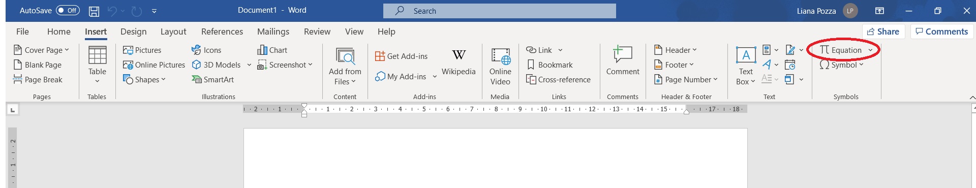
To Start off, open a word document, select the Insert tab and click your cursor on the Equation icon outlined in red in the screenshot below. This may look slightly different depending on the version of Word you are using.

Screenshot of Excel Equation tool highlighted

This will open up a menu (see screenshot below) for writing equations which is quite intuitive for most forms of equations.

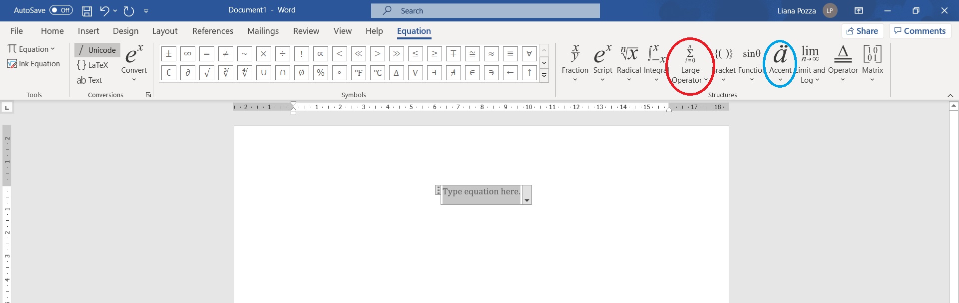
Screenshot of Excel Equation menu with Large Operator & Accent highlighted

The screenshot has outlined some less intuitive parts of equation you will need, the red outline is for equations requiring sigma notation (\sigma) such as the population variance, and outline in blue is for equations with accents such y-bar (\bar{y})for the sample mean and y-tilde (\tilde{y}) for the sample median.

Use MS Word to type the following equations

Mean:\bar{x} = \frac{1}{n} \sum_{i=1}^{n}x_{i}
Variance:\sigma^{2} = \frac{\sum\limits_{i=1}^{n} \left(x_{i} - \bar{x}\right)^{2}} {n-1}
The equation for a straight line:y = mx + b

You will also learn a little bit about how to write equations in R Studio using LATeX during this course.

Introduction to MS Excel

Excel has limited statistical capabilities but is quite useful for storing and manipulating small data sets. Due to the global dominance of MS Windows it is also the most commonly used format for storing and distributing data within workplaces so a super useful skill to have. While we will mostly be using RStudio in this course we will also be providing some exercises in MS Excel to help you get familiar with the software.

Excel worksheets and cells

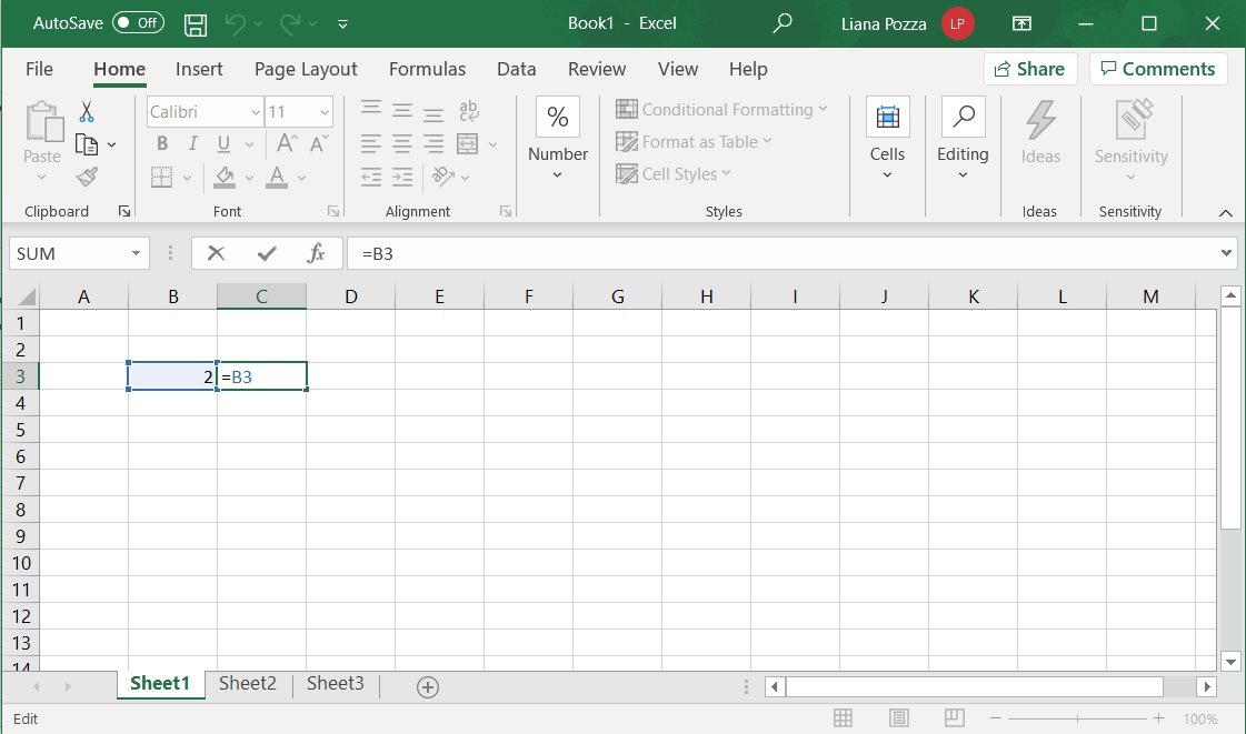
Excel files come in series of worksheets where data is stored in cells. The columns are given letters and the rows are given numbers, enabling a particular cell to be referenced by a combination a letter and number. In the screenshot below the number 2 in the orange cell could be referenced by B3. In a blank worksheet type 2 in the B3 cell.

In cell C3 type =B3

The equals sign tells Excel you are calculating something or referring to a cell. You should now have 2 in cell C3.

Screenshot of Excel Typing number 2 in cell B3

At the bottom of the Excel page you will see references to each of the worksheets in the file, for example ‘Sheet1’, ‘Sheet2’, ‘Sheet3’. This enables you to store multiple data sets in the one file. In this unit the data sets for each exercise will be stored in separate worksheets but in the same file.

Basic arithmetic in Excel

When typing equations, make sure you start by typing = . This tells Excel you want to solve the input equation.

The basic arithmetic operators return numeric values:

Key	Operation
+	Addition
-	subtraction
*	Multiplication
/	Division
^	Exponentiation

These can be used in combination with numbers or cell references.

For example, to get a value of 4 in cell D3 you can type either

=2*2 (type numbers)

=B3*C3 (reference cells)

It is better to reference cells so that if you change the values the same equations can be applied.

Basic functions in Excel

Some basic functions are:

Function	Operation
SUM	Sums a range of cells
COUNT	Counts a range of cells
LN	Natural Log
EXP	Exponent

These can be used in combination with numbers or cell references.

For example in cell E3 you can type either

=EXP(4) or =EXP(D3),

Another example is in cell F3 type

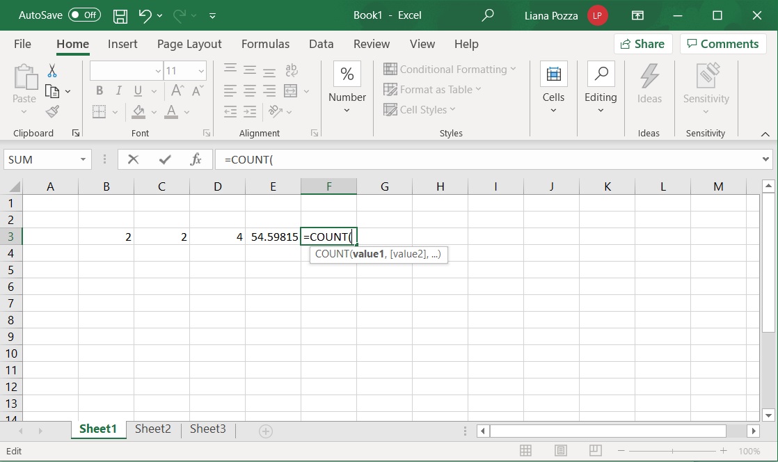
=COUNT(B3:D3)

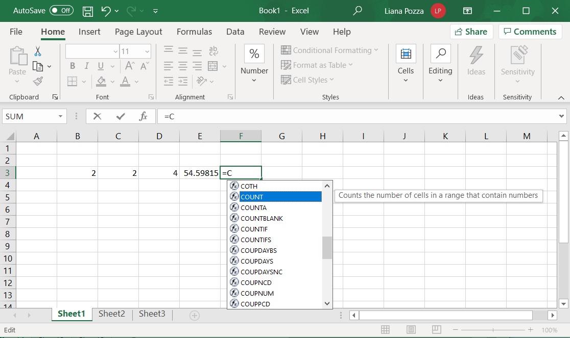
Note that Excel has an auto-complete function that allows you to select from a list of functions after typing the first letter i.e. =C. Selecting the function gives a brief description of what the function does.

Screenshot of Excel Typing =C to show function description

Once the function has been selected, you can proceed to type the opening bracket and enter in the cell reference, cell range or numeric value. Excel aids you in showing what the required input is as you type the opening bracket (see image below). The square bracket indicates an optional value, in this case if only one cell is selected =COUNT(E3), then the function will return the value 1.

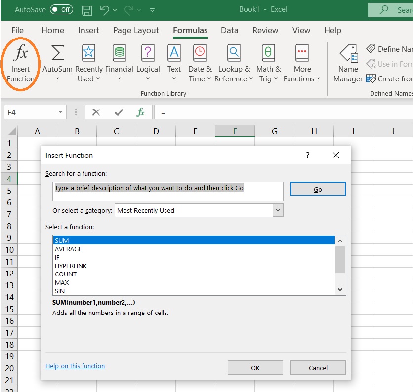
Screenshot of Excel showing required input arguments for COUNT function

Simple summary statistics in Excel

There are functions for calculating summary statistics in Excel. Click on a cell where you want the answer to be entered and then use the menu by Formulas >> Insert Function. A screenshot for calculating the sum is shown below.

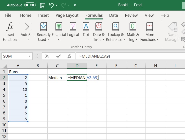
On the next screen you can then select the cells where the observations are located from which then median will be calculated.

After a while you should get to know the name of the functions in Excel and be able to write the arguments in manually. In the screenshot below the function is MEDIAN and it refers to cells between (and including) A2 and A9. A row or column of cells can be represented by the starting cell, then colon, then final cell (A2:A9).

Screenshot of Excel calculating the Median of cells A2 to A9

Some of examples of the functions that can be accessed in Excel are shown below. Note that the .S and .P extensions for variance and standard deviation are from later excel versions.

Statistic	Function
Minimum	=MIN
Maximum	=MAX
Arithmetic mean	=AVERAGE( )
Median	=MEDIAN( )
population variance	=VAR.P()
Sample variance	=VAR( ) or =VAR.S()
Population standard deviation	=STDEV.P()

Calculating simple summary statistics in Excel

In this exercise you will use the Lead_content.csv See start of lesson for link to download the file.

This data was collected from a recreational parkland in Sydney and is a measurement of the lead concentration (mg/kg) detected in the soil, measured through chemical analysis (ICP-OES). There are a total of 60 samples collected from around the park. The park was originally a municipal landfill but remediated in 1990, so we expected to find low levels of lead. The guide value set by the Australian Government is 300 mg/kg and this is where further investigation is needed (potential to cause harm).

In excel, calculate the following:

minimum value
Maximum value
mean
median
range
sample variance
sample standard deviation

From these statistics,

Were there any samples higher than the guide value?
Were there any samples where no lead was detected?
What is the mean value?

Introduction to R coding

R is a statistical programming language that can be used to store, manipulate, visualise and analyse data. It contains a number of pre-defined analysis techniques but you can also program your own methods.
R is open source which means that you can examine and modify the raw software code if you like. A worldwide collective of scientists, programmers and statisticians are working on improving and extending the capabilities of R.
Of immediate value to you is that it is free so for the rest of your career you can keep using R without burdening future employers with software licence fees. An article on the merits of R can be found by at http://monkeysuncle.stanford.edu/?p=367.
This module will provide an introduction to R. Work through the examples by typing in all code you see to familiarise yourself with the syntax of R and some of the commands available in R.

Getting a copy of R & RSudio

Remember that:

R = Engine and RStudio = Interface

Both are free & opensource and downloadable from https://posit.co/download/rstudio-desktop/.

Make sure you have installed both - it is best to have the latest version of R and RStudio. If you have not done this yet, please do so now.

R basics

To begin with we are going to open R (“The Engine”) from the program files menu on your computer.
When you open R, a window containing the R console will open. It will look slightly different depending on the operating system you use. The screenshot is from a Mac.

At the bottom of the screen is the command prompt >. Commands are typed at the command prompt and followed by the ENTER key.
From now type all the command you see into R. If you type in an expression, when you hit the ENTER key, the expression will be evaluated and the result returned, for example, lets add 5 and 5 together.

5+5

[1] 10

R is an object-oriented programming language and the basic unit in R is called an object. Objects can store single numbers, columns of data, modelling output, functions and other kinds of information.
The class of the object determines the way in which commands are executed on an object and the way in which data can be stored by the object. For example, vectors store a single column of data, a matrix can store multiple columns of data and a data frame can store multiple columns of data where the columns may be of different data types (e.g. numbers and text).
We can also save our result above into a named object using the assignment operator <- or =. I like the arrow because it points in the direction of the object being created. For example, the following command saves the value 5+5 as an object called myData.

myData <- 5+5

You can view the contents of an object by typing the object name:

myData

When you hit the RETURN Key, you will see the following output:

[1] 10

Object names can be made up of letters, numbers and , and _ symbols. A name must start with . or a letter. If it starts with . the second character must not be a number.
R is case sensitive, so calling mydata is not the same as myData and will generate an error:

mydata

Error in eval(expr, envir, enclos): object 'mydata' not found

To see a list of all the named objects you’ve created in R, use the objects function:

objects()

[1] "myData"          "pandoc_dir"      "quarto_bin_path"

To delete an object, use the remove function:

remove(myData)

If you type and enter an incomplete command, a continuation prompt will appear on the next line: +. You can continue typing the command followed by the ENTER Key.

myData3 <-
+ 8

To cancel a command at the continuation prompt (or during execution of a command), press the ESC key.
The up and down arrow keys can be used to scroll through previous commands.
Comments can be indicated by a hash mark (#) - everything on the line following the hash mark will be ignored by R. This can be after R code on a line or on a separate line as shown below.

#I am adding 6+6 and saving it to an object called my.Data
my.Data <- 6+6

Basic arithmetic in R

The symbols for basic arithmetic operators are shown in the table below.

Operators	Operation
+	addition
-	subtraction
*	multiplication
/	division
^ or **	exponentiation

Parentheses ( ) can be used to specify order of operations.
You can perform basic calculations by typing expressions into the command line.

(5*10) ^2

[1] 2500

Better still you can assign results to a named object to be used at a later date.

myresult <- 20/10 + 6 - 1

For example, We can then halve the value of myresult.

myresult <- myresult/2

Text editors in R

Until now you have copied and pasted commands which you may wish to use again. This is particularly important as you begin to write series of commands to perform a certain task. One option is to save these commands to text files and copy the relevant commands into R as needed. You can save logical groupings of commands into different text files.
A better option is to use text editors – one example is RStudio and unlike notepad it allows syntax highlighting of R commands. When an R session is open, RStudio includes an additional menu and toolbar and it allows the user to interact with R by submitting code in whole or in part.
From now on you should start to use RStudio by copying the commands into a R file and then submitting them to R. By doing this you will have a record of the commands you have used. From now you will be using R through RStudio and not the console directly. Over time you will develop a library of code to perform analyses and create graphics.
The screenshot below shows RStudio, the top left window shows your code and the bottom left window shows the input and output in R. The top right hand window side shows the objects you have created, for example myData. The bottom left hand corner shows graphics, in this case a histogram, but can also show other useful features such as the help menu.

Simple data analysis in RStudio

Download and open the file Code_Topic1.r see link at start of lesson. Once open using the File > Open menu items in RStudio, you will see most of the commands you have been typing in the code editor. Rather than typing commands directly into into R we will now start to use RStudio code editor.
You send code from your open R code file which the top left hand pane of to the R console which is found in the bottom left hand pane. The output, e.g. the mean, will also appear in the bottom left hand window.
To send a line of code to R from your R file (the Code_Topic1.R file), click anywhere in the line and click on the Run icon or use the short cut CTRL+ENTER (Windows) or COMMAND+ENTER (Mac) or click on Run to run all code at once. The output is shown in the bottom left hand window.
You can also use the # symbol to write comments which R will ignore. It is really important to comment throughout your code to help you and others who may use it to understand what the code does. It is recommended you copy the output into your R file and comment it out using # so you have a complete record of your work.

Getting data into RStudio

RStudio can accept data from many different sources; for example directly from scientific instruments or even scraping the internet for data. In this topic we are only considering small data sets so we will enter the data manually via the keyboard.
A vector (or list) of numbers can be manually entered using the assignment operator and the c function which essentially means combine, an example is below.

myDataset <- c(5,12,52,32,14,6.1)

Now it is your turn. Similar to above, use the c function to enter a soil carbon data set (48, 56, 90, 78, 86, 71, 42) as an object called Carbon. We will then calculate some basic statistics on this data set.

Carbon<-c(48, 56, 90, 78, 86, 71, 42)

Summary statistics in RStudio

Now we have entered the data in R we want to do something with it, such as calculate summary statistics.
R functions behave differently depending on the data type.
Some functions will work only on specific data types, other functions will use different methods on different data types.

To find the mean of data set we use the mean function.

mean(Carbon)

[1] 67.28571

Other commands related to summary statistics include:

median - median
var - sample variance
sd - sample standard deviation
min - minimum value
max - maximum value
length - number of observations (length of the vector)

Calculate all of the statistics above using R.

median(Carbon)

[1] 71

var(Carbon)

[1] 355.5714

sd(Carbon)

[1] 18.8566

min(Carbon)

[1] 42

max(Carbon)

[1] 90

length(Carbon)

[1] 7

Rather than using all of these indiviudally you can use the summary function which gives the minimum, maximum, mean and median values. We will consider the 1st Qu. and 2nd Qu. in the next practical.

summary(Carbon)

   Min. 1st Qu.  Median    Mean 3rd Qu.    Max. 
  42.00   52.00   71.00   67.29   82.00   90.00

Note, that it does not calculate the standard deviation, variance or number of observations.
That is all we will do in R in this practical. Remember to save your code so you can refer and reuse this for your online quiz and other assessments in the future.

Setting up a project in R and coding in Quarto

Working smartly with your data and code can save you time and tears. We are going to work with projects as this helps manage your data in a clean and easy way. You can either decide to creat a new project for each lab or create one project for the course.

Projects

Having all your files organised into a logical folder structure will be super beneficial in this course and also your day-to-day life. Also Super important is that you back up your work in the cloud. You can do this using One Drive which you can access as through your university account, you can also use your own cloud storage (Dropbox, iCloud,…) and or you can use your GitHub account.

Your tutors can assist you to get your files organised. The following is my recommendation:

Set up a course folder called ENVX1002 on your desktop/network drive/USB/cloud storage.
Set up a project folder called Lab_1 in your ENVX1002 folder.

Create a folder called ENVX1002 on your laptop or the class desktop (prefereably in a folder backed up to the cloud. If you are using a class computer you will need to save the file to upload to your cloud storage or USB/External Hard Drive or zip the folder and email to yourself at the end of the class.
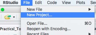
Open R Studio go to the file drop down menu and select New Project

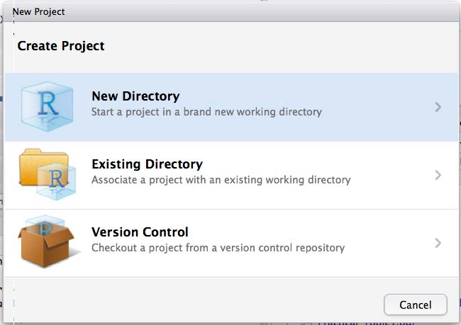
Select New directory and navigate to your class folder.

Enter on the directory name, for example Lab_1, and click on Create Project.
Well done! you have now set up a project.

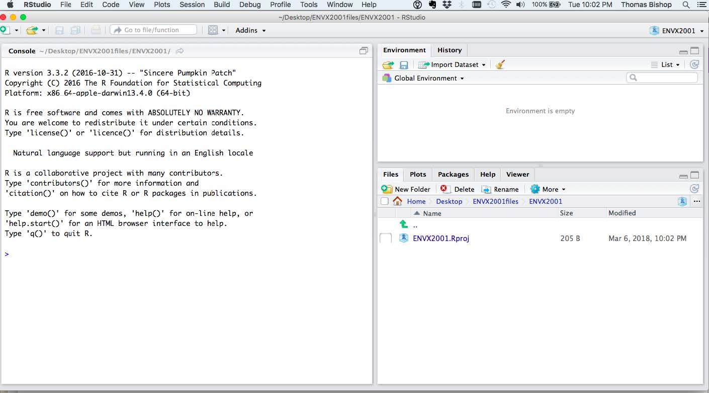6. You should now see a folder called Lab_1 in your ENVX1002 folder. If you open that folder you will see a file called Lab_1.Rproj. This is your project file and it will open RStudio with the working directory set to the Lab_1 folder.

Coding in Quarto

Your tutor will assist you to open a Quarto (.qmd) file. You will do this for each Lab and your also for your reports:

Open a qmd file, and save it as, for example, Prac1.qmd.
Run the file using render.
View filename.html in a browser.
Now experiment with editing the file (both text and code chunks) and then re-run using render.
Use this file to store your summary of today’s lab work.

The screenshots will help you do this.

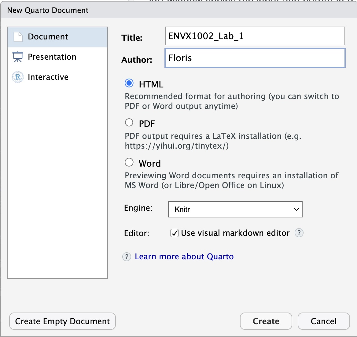
Navigate to New File > Quarto Document
Enter in an appropriate name for your file such as ENVX1002_lab_1 and enter in your name. Select HTML format.

Well done! you have created a new Quarto file. First save your file by navigating to the File menu i.e. File > Save as. Name your file ENVX1002_lab_1.qmd it should automatically save in your Project folder.
Finally you can Render the file by selecting the render button - see if you can spot it - it’s a blue block arrow pointing to the right above the text editor.
Go to your project folder and open the HTML file by double clicking on it, it will open in your default browser.

Summing up

Well done!

You now know how to:

write equations in a word document
do basic operations in Excel
do basic operations in R and RStudio and
consider how to manage files and folders and
set up a project as well as generate an Quarto Document

To do by next week:

complete anything you have missed from today’s lab
complete the practice O-quiz - this is to help you get familiar with Canvas quizzes.