Rows: 20
Columns: 3
$ extra <dbl> 0.7, -1.6, -0.2, -1.2, -0.1, 3.4, 3.7, 0.8, 0.0, 2.0, 1.9, 0.8, …
$ group <fct> 1, 1, 1, 1, 1, 1, 1, 1, 1, 1, 2, 2, 2, 2, 2, 2, 2, 2, 2, 2
$ ID <fct> 1, 2, 3, 4, 5, 6, 7, 8, 9, 10, 1, 2, 3, 4, 5, 6, 7, 8, 9, 10Topic 8 – A modern approach to hypothesis testing with infer
ENVX1002 Statistics in Life and Environmental Sciences
Floris van Ogtrop
The University of Sydney
Apr 2026
Announcement
- Practice Skills assessment this week, run in your respective labs. You must attend your lab to complete the assessment.
- A reminder that you are allowed to use cheat sheets for the assessment, but you must write or print them yourself
- maximum 2 sides of A4 paper
- no electronic devices allowed
- Printing services are available on campus. See here.
Learning Outcomes
By the end of this lecture, you can:
- Understand hypothesis testing as a comparison to a distribution
- Use simulation to generate that distribution from data
- Perform a hypothesis test using the infer package
- Interpret results without relying on strict assumptions
The Big Idea
How do we usually test hypotheses?
- Compare our observed result to a theoretical distribution
- This distribution is based on assumptions about the data (e.g., normality, equal variances)
A different idea
What if we didn’t assume a distribution at all?
- Use the data to simulate the distribution of the test statistic under the null hypothesis
- Simulate “no effect” data by randomly shuffling group labels (permutation test)
- Compare our observed statistic to this simulated distribution to get a p-value
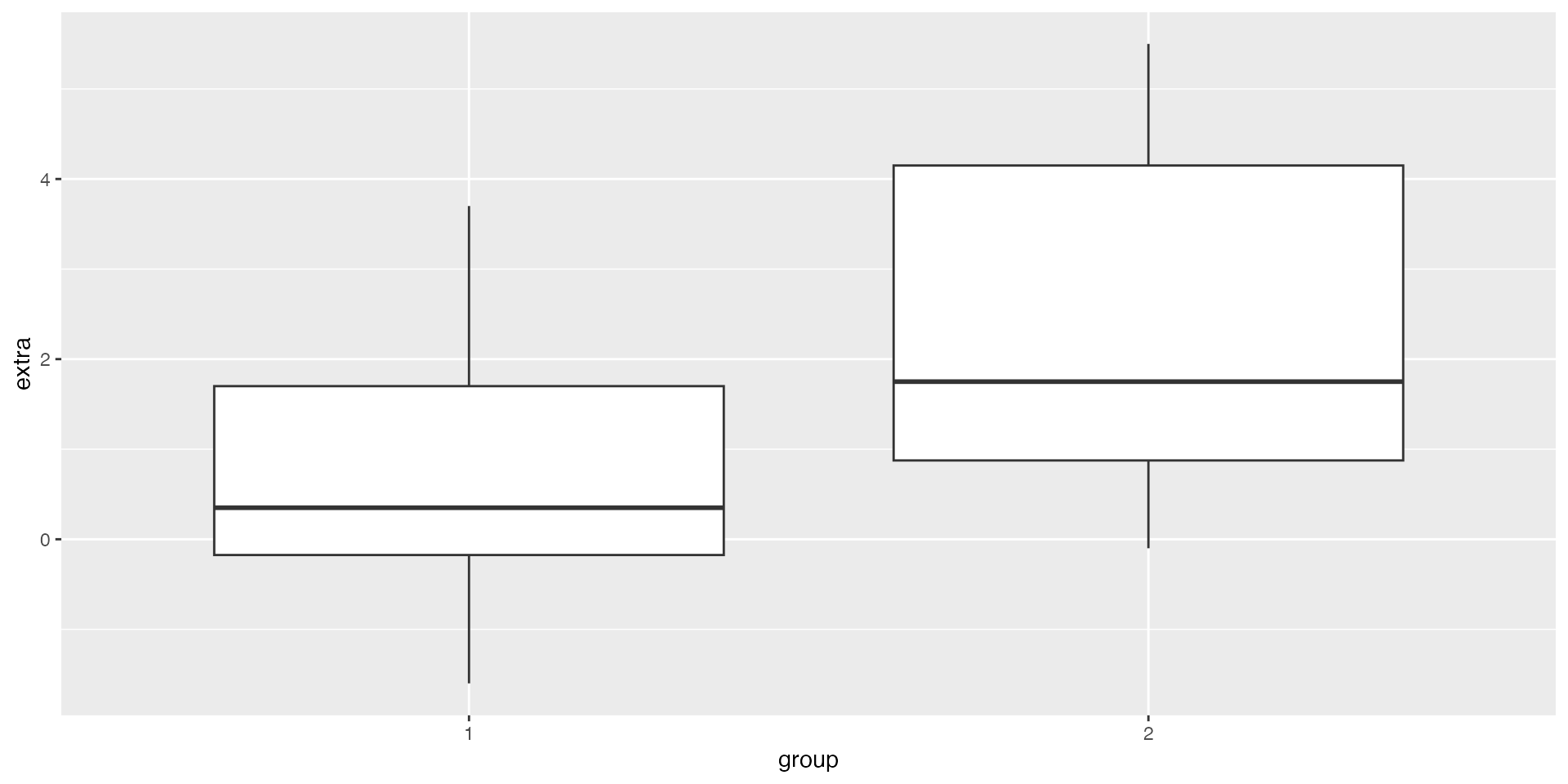
Example: Sleep data
Step 1 — Plot the data (EDA)
Step 2 Observed effect
- Create an observed test statistic using the infer workflow
- Take the ‘sleep’ dataset and pass it into the infer pipeline
- Define the response variable (‘extra’) and explanatory variable (‘group’) i.e., we are comparing ‘extra’ across the two groups
- Compute the statistic of interest: difference in group means
- Specify the order: mean(group 1) - mean(group 2). This determines the direction (sign) of the difference
Think first (Prediction)
Before we run the test:
- Does the difference look big or small?
- Do you expect:
- Small p-value (< 0.05)
- Moderate (~0.1)
- Large (> 0.2)
Commit to an answer
Step 3 — Simulate null distribution (HAT)
- Start with the dataset (sleep) to build a null distribution
- Set the seed for reproducibility
- Specify the response (extra) and grouping variable (group)
- (H) State the null hypothesis of no relationship (independence) - Assume the response is unrelated to group (i.e., group labels don’t matter).
- (A) Randomly shuffle group labels 1000 times to simulate “no effect” data (exchangeability under the null hypothesis)
- (T) Calculate the difference in means for each simulated dataset
Step 3 — p-value (P)
# A tibble: 1 × 1
  p_value
    <dbl>
1 0.076- we can visualise the null distribution and see where our observed statistic falls, and shade the area corresponding to the p-value
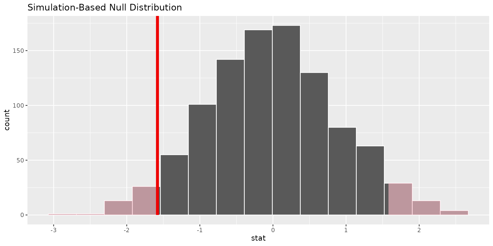
Conclusion (C)
If the observed statistic is rare under “no effect” → evidence against null In this case it is not super rare, so we do not have strong evidence against the null hypothesis of no difference in sleep between the two groups.
Compare to t-test
- The t-test also tests the null hypothesis of no difference between groups, but it relies on assumptions (e.g., normality, equal variances).
- The permutation test we performed does not rely on these assumptions and is based on the actual data.
- The p-value from the permutation test may differ from the t-test, especially if the assumptions of the t-test are violated. In this case, we might find that the t-test gives a different p-value, which could lead to a different conclusion about the evidence against the null hypothesis.
    Welch Two Sample t-test

data:  extra by group
t = -1.8608, df = 17.776, p-value = 0.07939
alternative hypothesis: true difference in means between group 1 and group 2 is not equal to 0
95 percent confidence interval:
 -3.3654832  0.2054832
sample estimates:
mean in group 1 mean in group 2
           0.75            2.33
Summary
Key points
- Hypothesis testing = compare to distribution
- We can simulate that distribution
inferprovides a clean workflow
simulate → compare → conclude
Final Thought
We are not memorising tests
We are learning how to “build” inference
Thanks!
This presentation is based on the SOLES Quarto reveal.js template and is licensed under a Creative Commons Attribution 4.0 International License.