Welcome!
This week we will test ANOVA assumptions using residual diagnostics, perform post-hoc comparisons with Tukey’s test, and practise back-transforming log-scale results using three datasets: diatoms, fish prolactin, and broiler chickens.
You will come across two types of tasks in this lab. Worked Examples have solutions you can expand and check straight away. Exercises do not — solutions for these will be posted on Friday evening.
Learning outcomes
In this lab, we will learn how to:
- Test the assumptions of ANOVA using residual diagnostics.
- Use plotting and Tukey’s tests to determine which pairs of groups are significantly different.
- Use R to perform the analyses.
Specific goals
By the end of this lab, you should be able to:
Preparation
This lab uses readxl, emmeans, and performance. Install any you are missing by running the following in the console:
Downloads
| File | Used in | Download |
|---|---|---|
Data4.xlsx |
All sections | Download |
Save the file into a folder called data inside your project folder.
1. Diatom diversity in streams (~20 min)
Here we will test the assumptions using residual diagnostics and finding significant differences using plots and Tukey’s test. The data is found in the Diatoms worksheet.
Testing assumptions and finding differences
Worked Example 1
Import the Diatoms worksheet from Data4.xlsx, convert Zinc to a factor, and fit a one-way ANOVA model.
tibble [34 × 4] (S3: tbl_df/tbl/data.frame)
 $ Stream   : chr [1:34] "Eagle" "Blue" "Blue" "Blue" ...
 $ Zinc     : Factor w/ 4 levels "BACK","HIGH",..: 1 1 1 1 1 1 1 1 3 3 ...
 $ Diversity: num [1:34] 2.27 1.7 2.05 1.98 2.2 1.53 0.76 1.89 1.4 2.18 ...
$ Group : num [1:34] 1 1 1 1 1 1 1 1 2 2 ... Df Sum Sq Mean Sq F value Pr(>F)
Zinc 3 2.567 0.8555 3.939 0.0176 *
Residuals 30 6.516 0.2172
---
Signif. codes: 0 '***' 0.001 '**' 0.01 '*' 0.05 '.' 0.1 ' ' 1Worked Example 2
Statistical test of the assumption of constant variance.
Statistics is made up of different tribes and some tribes use hypothesis testing to see if a dataset meets the assumptions of normality and constant variance. One option is the Bartlett’s test for constant variances. The mechanics are not important but the function and syntax are shown below. The hypotheses are:
H_0:\ \sigma_{BACK}^2=\sigma_{LOW}^2=\sigma_{MED}^2=\sigma_{HIGH}^2
H_1:\ not\ all\ \sigma_i^2\ are\ equal\ \left(i\ =\ BACK,\ LOW,\ MED,\ HIGH\right)
We prefer to use numerical and graphical diagnostics, e.g. residuals plots, but this is more to show you other possibilities. You can use this as a different line of evidence for testing assumptions if you wish.
Bartlett’s test will not work if the data is non-normal and only use it if the data has one treatment factor with a completely randomised design.
    Bartlett test of homogeneity of variances

data:  rstandard(anova.diatoms) by diatoms$Zinc
Bartlett's K-squared = 0.25337, df = 3, p-value = 0.9685
Based on the P-value being > 0.05 we could state that we retain the null hypothesis and that the variances are equal.
Worked Example 3
In Topic 3 we used the emmeans package to extract means for each group and their associated 95% CI. The emmeans is useful to produce a plot showing the mean and 95% CI which is a nice way to present the results.
 Zinc emmean    SE df lower.CL upper.CL
 BACK   1.80 0.165 30    1.461     2.13
 HIGH   1.28 0.155 30    0.961     1.60
 LOW    2.03 0.165 30    1.696     2.37
 MED    1.72 0.155 30    1.401     2.04

Confidence level used: 0.95 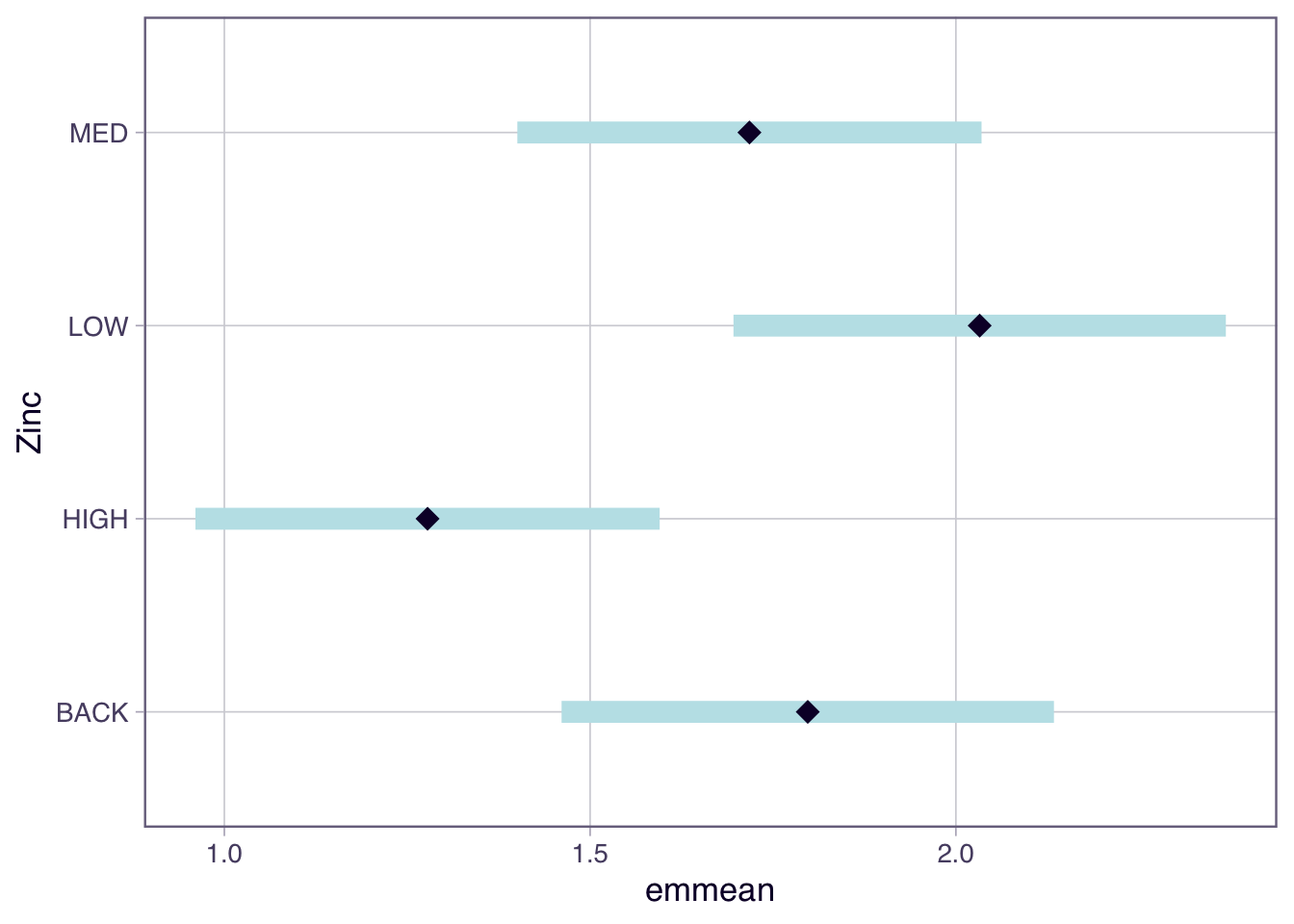
Based on the non-overlapping confidence intervals the only pairs of groups that are significantly different are HIGH and LOW. However more correctly we are looking at whether the difference in means = 0 which is a slightly different question to seeing if the 95% CI around the mean overlaps.
Worked Example 4
Another approach is to use a Tukey’s test which we can extract using the emmeans(model-goes-here, pairwise ~ your-treatment) function from the emmeans package. Note there are many other post-hoc tests that have come and gone, but we will just focus on one of them.
Another way to present the results is to use the plot() function to show the confidence intervals and the comparisons among them.
$emmeans
 Zinc emmean    SE df lower.CL upper.CL
 BACK   1.80 0.165 30    1.461     2.13
 HIGH   1.28 0.155 30    0.961     1.60
 LOW    2.03 0.165 30    1.696     2.37
 MED    1.72 0.155 30    1.401     2.04

Confidence level used: 0.95

$contrasts
 contrast    estimate    SE df t.ratio p.value
 BACK - HIGH   0.5197 0.226 30   2.295  0.1219
 BACK - LOW   -0.2350 0.233 30  -1.008  0.7457
 BACK - MED    0.0797 0.226 30   0.352  0.9847
 HIGH - LOW   -0.7547 0.226 30  -3.333  0.0117
 HIGH - MED   -0.4400 0.220 30  -2.003  0.2096
 LOW - MED     0.3147 0.226 30   1.390  0.5153

P value adjustment: tukey method for comparing a family of 4 estimates
You will note the following pairs are different:
- ‘LOW’ and ‘HIGH’;
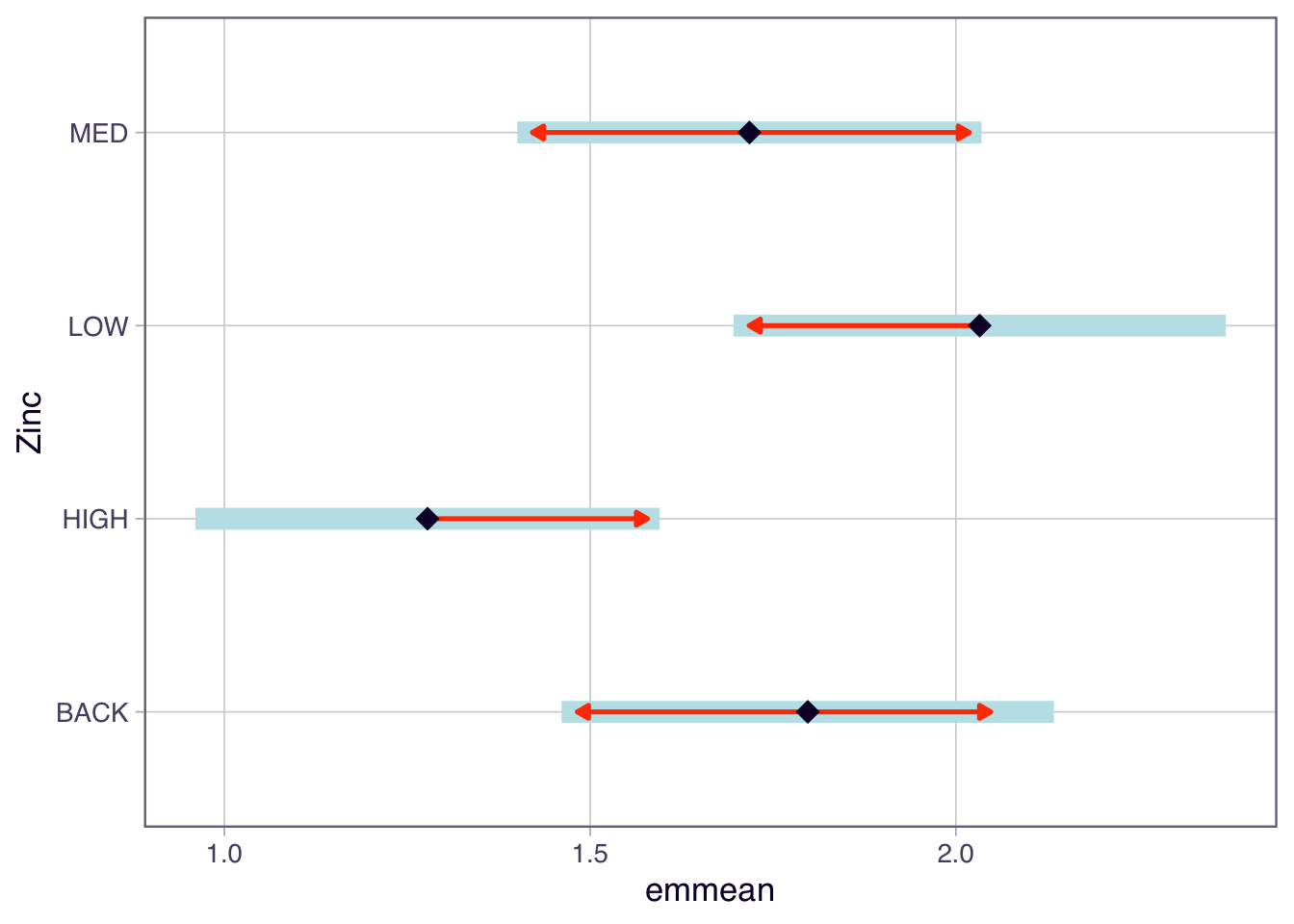
In the plot function above, we have specified comparisons = TRUE. The blue bars are confidence intervals for the EMMs, and the red arrows are for the comparisons among them. If an arrow from one mean overlaps an arrow from another group, the difference is not significant.
Worked Example 5
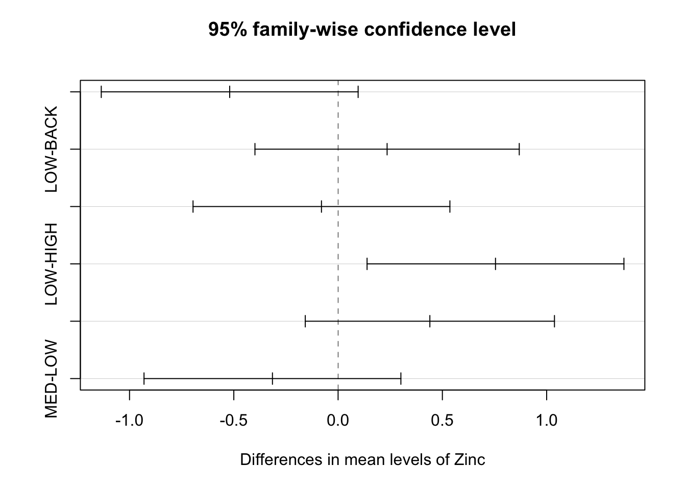
An alternative base R function for Tukey tests is TukeyHSD(). It creates a set of confidence intervals on the differences between the means of the levels of a factor. Also plot the results from this function.
If the confidence interval does not cross over 0, then that pair significantly differs from each other.
  Tukey multiple comparisons of means
    95% family-wise confidence level

Fit: aov(formula = Diversity ~ Zinc, data = diatoms)

$Zinc
                 diff        lwr        upr     p adj
HIGH-BACK -0.51972222 -1.1355064 0.09606192 0.1218677
LOW-BACK   0.23500000 -0.3986367 0.86863665 0.7457444
MED-BACK  -0.07972222 -0.6955064 0.53606192 0.9847376
LOW-HIGH   0.75472222  0.1389381 1.37050636 0.0116543
MED-HIGH   0.44000000 -0.1573984 1.03739837 0.2095597
MED-LOW   -0.31472222 -0.9305064 0.30106192 0.5153456
We can also plot the results from TukeyHSD() to easily see where, if any, the differences are.
Note a type I error rate is defined by your significance level (alpha). In other words, there is a chance that you will reject a null hypothesis that is actually true — it is a false positive. When you perform only one test, the type I error rate equals your significance level, which is often 5%. However, as you conduct more and more tests, your chance of a false positive increases. If you perform enough tests, you are virtually guaranteed to get a false positive! The error rate for a family of tests is always higher than an individual test. Here in the TukeyHSD function you set the family-wise level of significance and the p-values for the individual tests are adjusted accordingly.
Before we move on, now is a good time to take a 5-minute break.
2. Prolactin in stickleback fish (~30 min)
In this exercise will add a layer of complexity by considering a transformation. If our data does not meet the assumptions we need to transform the data, possible transformations are the square root (weak) and log (high). When we transform the data we need to be careful about how we interpret the results.
Concentration of prolactin (units g/L) in the pituitary glands of nine-spined stickleback fish was assessed. The fish were kept in either saltwater or freshwater prior to assay and were different batches were examined on three successive occasions. Cysts tend to develop in fish when kept in saltwater and sometimes develop in freshwater populations. The four different groups of fish were used in a preliminary experiment to examine the effects of cysts, whether induced by saltwater or normally present, on the prolactin production of the pituitary gland.
The four groups of fish were codes as follows, with 10 fish per group:
A = saltwater cysts, day 1;
B = freshwater, no cysts, day 2;
C = freshwater, no cysts, day 2;
D = freshwater, cysts, day 3.
The data is found in the Prolactin worksheet.
Exploratory analysis and assumptions
Exercise 1
Import the data into R, perform some exploratory data analysis to make tentative suggestions about differences between means and the likelihood of the data meeting the assumptions.
Exercise 2
Fit an ANOVA model and test the assumption of normality using a QQ plot and a histogram - both based on standardised residuals.
Exercise 3
Assess the assumption of constant variance by:
- examine the plot of the standardised residuals against fitted values;
- From the performance package, use
check_model()to assess the assumptions of the model. This function will check the assumptions of normality and constant variance;
- using the Bartlett’s test;
- using
check_homogeneity()from theperformancepackage;
- calculating the ratio of the largest SD:smallest SD to see if it is below 2:1;
Note there are many tests: method = c("bartlett", "fligner", "levene", "auto")
Exercise 4
The data does not meet the assumptions so log transform (log function) the response and repeat the normality and constant variance checks to test the assumptions.
In R you can transform data in the model formula or you could create a new column in your data frame, for example fish$logProlactin <- log(fish$Prolactin).
Post-hoc tests and back-transformation
Exercise 5
If the assumptions are met and there is significant F-test perform Tukey tests and identify which pairs are significantly different.
Exercise 6
One issue is that we have performed our hypothesis testing on the log scale. This means there are some steps to be made if we wish to interpret the data on the original scale; e.g. provide a 95% CI on the original scale. We will step through these.
Suppose the biologist was primarily interested in comparing the prolactin concentrations for A (saltwater cysts, day 1) vs B (freshwater, no cysts, day 1).
- Find the means and CI from the output of the
TukeyHSD()oremmeans()function. - The CI and mean are on the log scale, so back-transform the difference in the means (
exp()function), the lower and upper end-point 95% CI. Note that the upper and lower tail are not of equal length on the original scale.
Now we have an estimate of the difference in the means on the original scale. It actually corresponds to a ratio on the original scale. The reason is based on log laws, we can write the difference between 2 logged numbers (A and B) as a log of their ratio (A/B);
\log\left(A\right)-\log\left(B\right)=\log\left(\frac{A}{B}\right).
If we back-transform the log of their ratio we get the ratio on the original scale;
e^{\log\left(\frac{A}{B}\right)}=\frac{A}{B}.
So the back-transformed difference between the pairs of the means is a ratio.
Note: if we were to back-transform the group means on the log scale we would get the geometric mean on the original scale.
Provide a biological interpretation for this estimate and confidence interval. Use the CI to decided if there is a significant difference between Treatment A and Treatment B.
Before we move on, now is a good time to take a 5-minute break.
3. Broiler chickens (~25 min)
This exercise is an analysis of a set of growth data. It is an open question for you to gain more practice.
The effect of weight gain in dressed broiler chickens was determined after five generations of selection. Group A was bred by using only the heaviest 10% in each generation; groups B and C were bred using respectively the heaviest 30% and 50%; group D was obtained by crossing groups A and C of the previous generation. The dressed weights (kg) of 25 birds from each group have been recorded.
The data is found in the Broilers worksheet.
Analysis
Exercise 7
Write down the null and alternate hypothesis. What is the treatment factor, and how many levels does it have? What are the sample sizes for each group (n_i)?
Exercise 8
Import the data into R, and then obtain some numerical and graphical summaries of the data, by each group. How would you interpret these data? From these summaries, is the assumption of homogeneity of variances met? What about normality? Try a formal Bartlett’s test using the bartlett.test or check_homogeneity() function. Use residual diagnostics to assess the assumptions.
Exercise 9
Note that the results of the analysis can only be used when the assumptions of the analysis have been met. If you believe that the assumptions are met, then what would your conclusions of the analysis of variance be? You should use the summary() function applied to your aov() object to obtain the ANOVA table.
Without any formal analysis, consider the result of the group means in relation to the group treatment - i.e. type of selection. Would this pattern be expected? If appropriate perform a Tukey test.
Conclusion
Closing thoughts
We tested ANOVA assumptions using residual diagnostics, applied transformations when assumptions were violated, and used post-hoc tests to identify which groups differ. These tools will be used throughout the rest of the course as we fit more complex models.
Attribution
This lab was developed using resources that are available under a Creative Commons Attribution 4.0 International license, made available on the SOLES Open Educational Resources repository.