Learning outcomes
In this lab, you will work towards achieving learning outcomes L03, and L05.
Lab objectives
In this lab, we will:
Please work on this exercise by creating your own R Markdown file.
Preparation
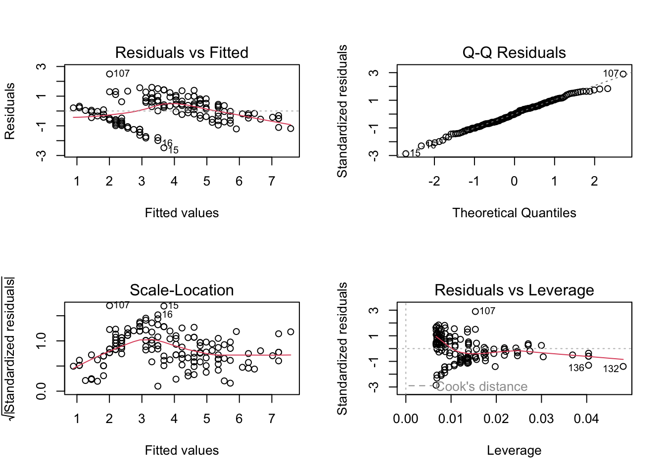
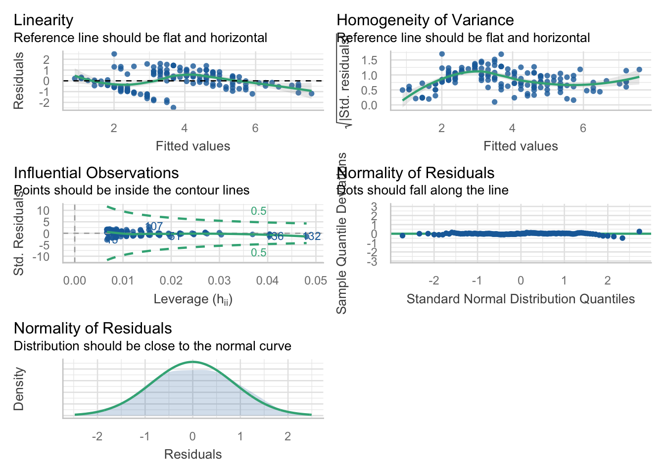
This package is really good for checking your models. For this lab, we will focus on the check_model() function, which gives us nice pretty diagnostic plots for models:
Exercise 1: Modelling bird abundance
We will now use the transformed data in loyn for this exercise. If you have not already figured out how to perform the transformation, or if something is wrong, you may use the loyn tab in the mlr.xlsx MS Excel document. Alternatively, the code to convert the data is below.
This is the same data we used in the walkthrough exercise
Rows: 56
Columns: 10
$ ABUND    <dbl> 5.3, 2.0, 1.5, 17.1, 13.8, 14.1, 3.8, 2.2, 3.3, 3.0, 27.6, 1.…
$ AREA     <dbl> 0.1, 0.5, 0.5, 1.0, 1.0, 1.0, 1.0, 1.0, 1.0, 1.0, 2.0, 2.0, 2…
$ YR.ISOL  <dbl> 1968, 1920, 1900, 1966, 1918, 1965, 1955, 1920, 1965, 1900, 1…
$ DIST     <dbl> 39, 234, 104, 66, 246, 234, 467, 284, 156, 311, 66, 93, 39, 4…
$ LDIST    <dbl> 39, 234, 311, 66, 246, 285, 467, 1829, 156, 571, 332, 93, 39,…
$ GRAZE    <dbl> 2, 5, 5, 3, 5, 3, 5, 5, 4, 5, 3, 5, 2, 1, 5, 5, 3, 3, 3, 2, 2…
$ ALT      <dbl> 160, 60, 140, 160, 140, 130, 90, 60, 130, 130, 210, 160, 210,…
$ L10AREA  <dbl> -1.0000000, -0.3010300, -0.3010300, 0.0000000, 0.0000000, 0.0…
$ L10DIST  <dbl> 1.591065, 2.369216, 2.017033, 1.819544, 2.390935, 2.369216, 2…
$ L10LDIST <dbl> 1.591065, 2.369216, 2.492760, 1.819544, 2.390935, 2.454845, 2…
Best single predictor?
Question 1
Obtain the correlation between ABUND and all of the predictor variables using cor(). Based on these, what would you expect to be the best single predictor of ABUND?
Assumptions and interpretation
Question 2
Use multiple linear regression to see whether ABUND can be predicted from L10AREA and GRAZE. Are the assumptions met? Is there a significant relationship? Note: we are using these 2 predictors as they have the largest absolute correlations. Use lm() and specify the model as ABUND ~ L10AREA + GRAZE.
Question 3
How good is the model based on the (i) r2 (ii) adjusted r2? Use summary().
Question 4
Which variable(s) has the most significant effect(s)? (Refer specifically to the t probabilities in the table of predictors and their estimated parameters or coefficients in the output of summary()). Interpret the p-values in terms of dropping predictor variables.
Question 5
Repeat the multiple regression, but this time include YRS.ISOL as a predictor variable (it has the 3rd largest absolute correlation). This will allow you to assess the effect of YRS.ISOL with the other variables taken into account.
Question 6
Check assumptions, do the residuals look ok? If you are happy with the assumptions, you can proceed to interpret the model output.
Question 7
Compare the r2 and adjusted r2 values with those you calculated for the 2 predictor model, Which is the better model? Why?
Exercise 2: California streamflow
The following dataset contains 43 years of annual precipitation measurements (in mm) taken at (originally) 6 sites in the Owens Valley in California. I have reduced this to three variables labelled lake_sabrina (Lake Sabrina), pine_creek (Big Pine Creek), rock_creek (Rock Creek), and the dependent variable stream runoff volume (measured in ML/year) at a site near Bishop, California (labelled runoff_volume).
Note the variables have already been log-transformed to increase normality of the residuals in the regressions.
Start with a full model and manually remove the variables one at a time, checking every time whether removal of a variable actually improves the model.
[1] "lake_sabrina" "pine_creek" "rock_creek" "runoff_volume"
Call:
lm(formula = runoff_volume ~ ., data = stream_data)

Residuals:
     Min       1Q   Median       3Q      Max
-0.09885 -0.03331  0.01025  0.03359  0.09495

Coefficients:
             Estimate Std. Error t value Pr(>|t|)
(Intercept)   3.25716    0.12360  26.352  < 2e-16 ***
lake_sabrina  0.05631    0.03756   1.499  0.14185
pine_creek    0.21085    0.06756   3.121  0.00339 **
rock_creek    0.43838    0.08798   4.983 1.32e-05 ***
---
Signif. codes:  0 '***' 0.001 '**' 0.01 '*' 0.05 '.' 0.1 ' ' 1

Residual standard error: 0.04861 on 39 degrees of freedom
Multiple R-squared:  0.8817,    Adjusted R-squared:  0.8726
F-statistic: 96.88 on 3 and 39 DF,  p-value: < 2.2e-16
Partial F-Tests
The above analysis tells us that both pine_creek & rock_creek are significant, according to the t-test, in the model and lake_sabrina is not? This involves performing Partial F-Tests as discussed in the lecture.
This can be done in R by using anova() on two model objects. To be able to compare the models and run the anova, you need to make objects of all the possible model combinations you want to compare.
The last row gives the results of the partial F-test.
Question 1
Should we remove lake_sabrina from the model?
Question 2
Is the p-value for the f-test the same as for the t-test?
Question 3
Write out the hypotheses you are testing.
Perform a Partial F-Test to work out if the removal of lake_sabrina and pine_creek improves upon the full model.
Analysis of Variance Table

Model 1: runoff_volume ~ lake_sabrina + pine_creek
Model 2: runoff_volume ~ lake_sabrina + pine_creek + rock_creek
  Res.Df      RSS Df Sum of Sq     F    Pr(>F)
1     40 0.150845
2     39 0.092166  1   0.05868 24.83 1.321e-05 ***
---
Signif. codes:  0 '***' 0.001 '**' 0.01 '*' 0.05 '.' 0.1 ' ' 1
Question 4
Which variable should be added to the model containing rock_creek?
Question 5
Could things be even simpler? Perform a partial F-Test to see if a model containing rock_creek alone could be suitable.
Question 6
What is your optimal model?
Review
Simple linear regressions model the relationship between two variables
- We can also make linear models with more than one predictor
We can use histograms and correlation matrices to do some preliminary exploration of the data
If any variables are skewed, we can transform them
Looking at a correlation matrix to identify the best predictors (for both simple and multiple linear regression)
Fit model using
lm()functionCheck assumptions:
- Collinearity (multiple linear regression only)
- Linearity
- Independence
- Normality
- Equal variance
Use
summary()to look at model output and interpret it- F-test : overall model significance
- Coefficients table : individual predictors’ significance
- R2 : How much variation in the data is explained by the model?
That’s it for today! Great work fitting simple and multiple linear regression! Next week we jump into stepwise selection!