Lecture 01a – Welcome

ENVX2001 Applied Statistical Methods

Januar Harianto

Lecturer, SOLES

Apr 2026

This is ENVX2001

Staff

A. Prof Aaron Greenville
Unit Coordinator
Weeks 4-6

Dr Liana Pozza
Lecturer
Weeks 7-9

Dr Januar Harianto
Lecturer
Weeks 1-3

Prof Mathew Crowther
Professor
Weeks 9-11

Your statistical journey

Does migration come at a cost?

In a partially migratory elk population in Alberta, Canada, researchers compared calf birth weights between resident and migrant herds.

Code
elk <- read.csv("data/elk_calf_clean.csv")
elk$mig_status <- factor(elk$mig_status,
  levels = c("Resident", "Eastern"),
  labels = c("Resident", "Migrant")
)

ggplot(elk, aes(x = mig_status, y = birth_wt, fill = mig_status)) +
  geom_boxplot(show.legend = FALSE) +
  scale_fill_viridis_d(end = 0.9) +
  labs(x = NULL, y = "Birth weight (kg)") +
  theme_minimal(base_size = 18)

You have already learnt to compare groups like this with t-tests (Weeks 1–3).

Can dogs smell human stress?

Eighteen pet dogs were exposed to odours from humans who were either relaxed or stressed. Researchers then measured how long each dog took to approach food bowls.

Code
dogs <- read.csv("data/dog_odour_clean.csv")
dogs$treatment <- factor(dogs$treatment,
  levels = c("Baseline", "Relaxed", "Stressed")
)

dog_means <- aggregate(latency ~ dog_id + treatment, data = dogs, FUN = mean)

ggplot(dog_means, aes(x = treatment, y = latency, fill = treatment)) +
  geom_violin(alpha = 0.6) +
  scale_fill_viridis_d(end = 0.9) +
  labs(x = "Odour treatment", y = "Mean latency (s)") +
  theme_minimal(base_size = 18) +
  theme(legend.position = "none")

What if there are more than 2 groups to compare? We use Analysis of Variances (ANOVA) (Weeks 3–6).

How big is that penguin?

Heavier penguins tend to have longer flippers – but how strong is that relationship?

Code
penguins <- palmerpenguins::penguins

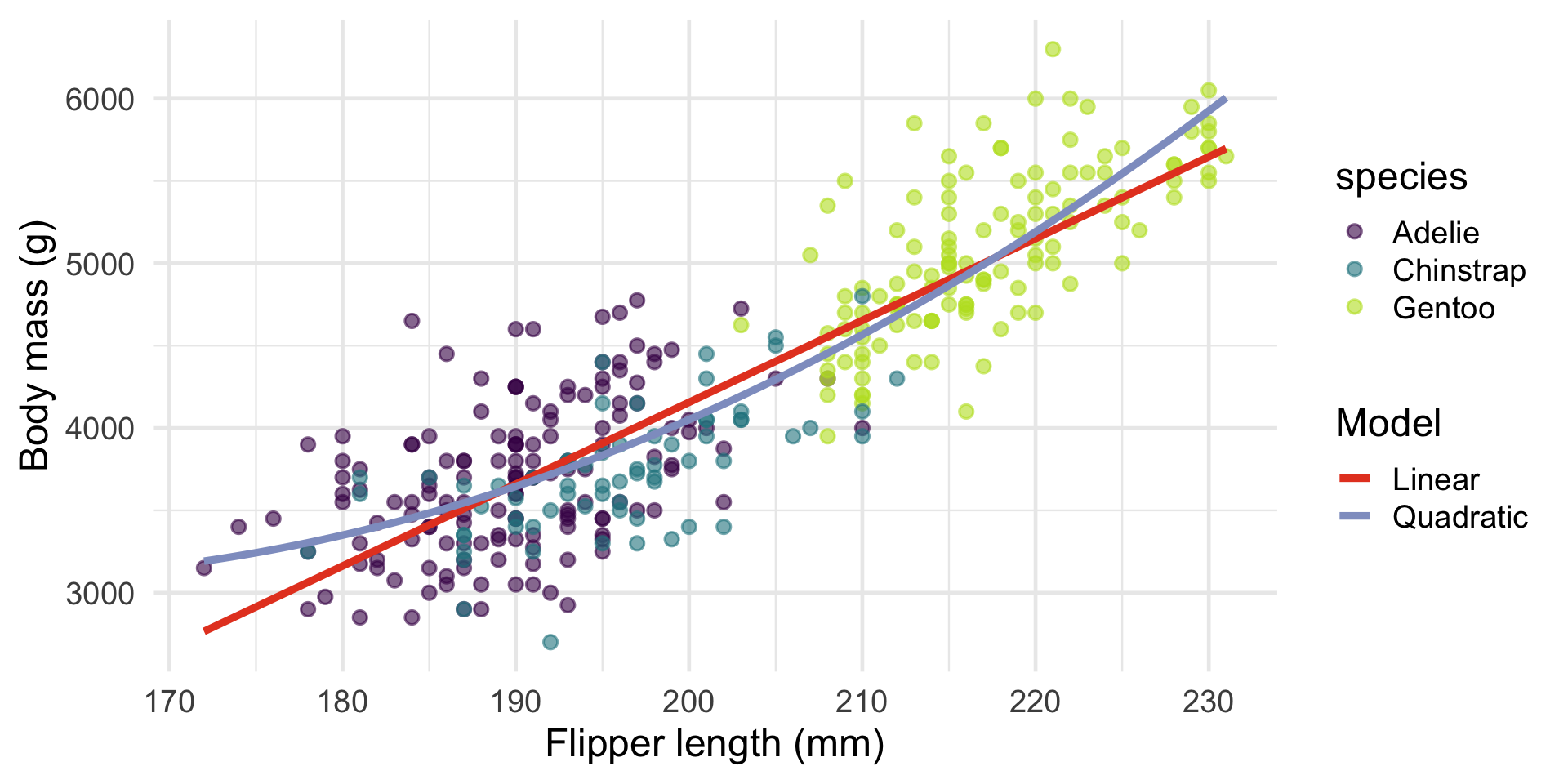
ggplot(penguins, aes(x = flipper_length_mm, y = body_mass_g)) +
  geom_point(aes(colour = species), alpha = 0.6) +
  geom_smooth(method = "lm", se = FALSE, colour = "#e64626", aes(linetype = "Linear")) +
  geom_smooth(method = "lm", formula = y ~ poly(x, 2), se = FALSE, colour = "#8f9ec9", aes(linetype = "Quadratic")) +
  scale_colour_viridis_d(end = 0.9) +
  scale_linetype_manual(values = c(Linear = "solid", Quadratic = "solid")) +
  guides(linetype = guide_legend(override.aes = list(colour = c("#e64626", "#8f9ec9")))) +
  labs(x = "Flipper length (mm)", y = "Body mass (g)", linetype = "Model") +
  theme_minimal(base_size = 18)

We can model this relationship with regression, but how do we validate this against other models? You will learn to do this with model selection (Weeks 7–9).

Hawks of Iowa

Researchers at Lake MacBride, Iowa trapped three hawk species over a decade and measured wing length, weight, culmen, and hallux on each bird.

Code
hawks <- read.csv("data/hawks_clean.csv")
pca <- prcomp(hawks[, c("Wing", "Weight", "Culmen", "Hallux")], scale. = TRUE)
scores <- data.frame(pca$x, Species = hawks$Species)

ggplot(scores, aes(x = PC1, y = PC2, colour = Species)) +
  geom_point(alpha = 0.5) +
  stat_ellipse(linewidth = 1) +
  scale_colour_viridis_d(end = 0.9) +
  labs(x = "PC1", y = "PC2", colour = "Species") +
  theme_minimal(base_size = 18)

We can represent multivariate data in fewer dimensions using multivariate methods (Weeks 10–12).

Housekeeping

Lectures

Wednesdays 10am - 12pm, Chemistry Lecture Theatre 3 (CLT03)

Copyright The University of Sydney

Labs

Labs are held at the South Eveleigh Precinct

Credit: Michael Wheatland

Directions from Carslaw

If the map does not load, click here

Transport options

Buses

Courtesy buses are available from Fisher Library to Redfern Station. You must then walk to the precint (10 minutes).

Driving

Free parking is available around Henderson Road, but it is extremely crowded. We do not recommend driving to the precinct.

Walking

Walking to the South Eveleigh Precinct takes about 20 minutes from Carslaw. You can save approximately 5 minutes by using Redfern station’s community access gates.

Expectations

Attendance

Lectures

  • You are expected to attend 80% of lectures
  • We may collect attendance data to determine if students are engaging with the course

Labs are compulsory with 80% minimum attendance

  • Labs are the heart of this unit. No exceptions except through special consideration
  • Attendance is recorded - we take attendance seriously and tutors may not record attendance for students who game the attendance system (e.g., signing in for a friend, leaving early without permission, etc.)

Assessments

Check Unit Outline

Week Assessment Weight Type
3 Early Feedback Task 1% Individual
5 Project 1: Describing data 10% Individual
10 Project 2: Analysing experimental data 20% Individual
13 Project 3: Presentation (multivariate) 20% Group
- Quizzes (weekly, multiple due dates) 4% Individual
- Exam (2 hours, MCQs + Short Answers) 45% Individual

Doing well

Put in the hours

  • This is a 6 credit point unit, which means that you are expected to spend 120 – 150 hours in total, including exam prep time (~10 h per week)!
  • Practice makes perfect. Tutorials and Labs help you apply the concepts you learn in lectures – complete all the exercises, and practice with the bonus questions provided.

Ask questions

Don’t be afraid to seek help. We are happy when students show genuine interest to learn and will do our best to support you. Here are some ways to ask questions:

  • Ed Discussion is the best place to ask questions. We are way more responsive on Ed than on email.
  • Drop-in sessions are available. Check Ed Discussion for times and links.

Learning outcomes

By the end of this course, we want you to be able to:

  • LO1 demonstrate proficiency in designing sample schemes and analysing data from them using R.
  • LO2 describe and identify the basic features of an experimental design: replicate, treatment structure and blocking structure.
  • LO3 demonstrate proficiency in the use or the statistical programming language R to apply an ANOVA and fit regression models to experimental data.
  • LO4 demonstrate proficiency in the use or the statistical programming language R to use multivariate methods to find patterns in data.
  • LO5 interpret the output and understand conceptually how its derived of a regression, ANOVA and multivariate analysis that have been calculated by R.
  • LO6 write statistical and modelling results as part of a scientific report.
  • LO7 appraise the validity of statistical analyses used publications.

Questions?

This presentation is based on the SOLES Quarto reveal.js template and is licensed under a Creative Commons Attribution 4.0 International License

Take a break

We will resume the second half of the lecture in 10 minutes. Come on down if you have questions!