Sampling designs… or why confidence intervals are important in stats
By the end of today
We will:
Calculate and interpret confidence intervals for a population mean
Compare simple random and stratified random sampling designs
Determine how to estimate change over time using monitoring data
Soil carbon
Estimating soil carbon
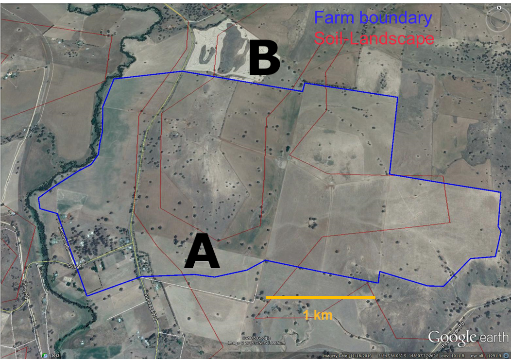
A farmer wants to estimate the average soil carbon on their property to apply for a carbon credit scheme. Their budget allows for 7 measurement sites.
Where should they sample, and how confident can they be in the result?
Observational studies
The farmer cannot change their land, so they measure it as it is. This makes their study an observational study.
Observational study
We measure the world as it is
Can show association, not causation
E.g. surveys, monitoring studies
Controlled experiment
We manipulate conditions
Can establish causation
E.g. clinical trials, field experiments
Two types of observational study
Right now, the farmer is taking a single snapshot of their property, a survey.
Later, they might return to measure again over several years, a monitoring study.
We will come back to monitoring in the second half.
Surveys
A snapshot at one point in time
Estimate a statistic (e.g. mean)
Measuring species richness in a forest
Monitoring studies
Multiple snapshots over time
Estimate a change in a statistic
Measuring species richness before and after a fire
Choosing where to sample
Simple random sampling
The farmer needs a plan for choosing their 7 sites. The simplest approach: simple random sampling.
Each unit has an equal chance of being selected.
Randomly sample units from the entire population.
Like putting all names in a hat and drawing some out randomly.
What is “random” sampling?
The farmer might be tempted to just walk to convenient spots, but that would bias the sample. Convenient locations are often atypical: near paths, buildings, or water sources.
So what makes a sample truly “random”?
Within a population, all units must have a probability greater than zero of being selected. Nothing can be excluded by design.
For simple random sampling, this probability is equal for every unit.
We call this probability the inclusion probability.
How do we achieve random sampling?
Random sampling requires a formal procedure, not just picking samples that “feel” representative.
Tools for random selection
Random number generator: for example, R’s sample() function
Random number table: a pre-generated list of random digits
The selection method must be reproducible and unbiased
Using R’s sample() function, the farmer randomly selects 7 grid cells from a map of their property.
The farmer collects data
The farmer uses simple random sampling to select 7 grid cells, then measures soil carbon at each site.
The measurements: 48, 56, 90, 78, 86, 71, 42 t/ha.
soil <-c(48, 56, 90, 78, 86, 71, 42)soil
[1] 48 56 90 78 86 71 42
How confident is the estimate?
The farmer’s mean
The farmer calculates the mean:
mean(soil)
[1] 67.28571
The result is 67.3 t/ha. But is this number the true average for the whole property?
How much should we trust an estimate?
Two studies both report a mean soil carbon of 67 t/ha. One measured 5 sites, the other 500.
Should we trust them equally?
The problem of a single estimate
A single number on its own does not tell us anything about uncertainty. We need a way to combine our estimate with how precise it is. That is what confidence intervals do.
A confidence interval (CI) gives us a range of plausible values for the population parameter, rather than a single best guess.
It combines three things:
Our estimate (the sample mean)
How precise that estimate is (the standard error)
How confident we want to be (the critical value)
Calculating confidence intervals
The three ingredients, formally
Sample mean (\(\bar{x}\)): our estimate of the population parameter
Standard error of the mean (\(SE_{\bar{x}} = s / \sqrt{n}\)): how precise that estimate is
Critical value (\(t_{n-1}\)): from the t-distribution at our chosen confidence level (e.g. 95%). We use t rather than the normal distribution because we estimate \(\sigma\) from the sample.
The \(t_{n-1} \times SE_{\bar{x}}\) part is the margin of error, the “plus or minus” value you often see in survey results (±3%).
To use this formula, we need to understand two things: degrees of freedom and the t-distribution.
Degrees of freedom
The farmer estimated one thing from their sample: the mean. That uses up one degree of freedom:
\[
\text{df} = n - 1
\]
For the farmer: \(df = 7 - 1 = 6\). This number determines which t-distribution we use, and therefore how wide the CI is.
Why \(n - 1\)?
Imagine you have 4 numbers with a mean of 5:
You can freely choose the first three numbers: 3, 10, and 7
But the fourth number MUST be 0 to make the mean equal 5: \((3 + 10 + 7 + 0) \div 4 = 5\)
So only 3 numbers (\(n - 1\)) can be freely chosen = 3 degrees of freedom
Why not use the normal distribution?
The farmer only has 7 samples, so they do not know the true population standard deviation. They have to estimate it from the sample, and that adds uncertainty.
The t-distribution accounts for this extra uncertainty. It has heavier tails than the normal, meaning more probability in the extremes.
The farmer’s \(df = 6\) gives a critical value of 2.447 (compared to 1.96 from the normal)
This makes the CI wider, which is more honest about how uncertain a small sample really is
With larger samples, the t and normal distributions converge, and the difference stops mattering around \(n = 30\)
The t-distribution in action
The solid curve is the t-distribution; the dashed curve is the normal. At \(df = 6\) (the farmer’s case), the tails are noticeably heavier. As \(df\) increases, the two curves converge.
Code used to generate the animation above
anim_speed <-1x <-seq(-4, 4, length.out =400)dfs <-c(1:5, seq(6, 30, by =2))t_curves <-do.call(rbind, lapply(dfs, function(df) {data.frame(x = x, density =dt(x, df), df = df)}))normal_curve <-data.frame(x = x, density =dnorm(x))p <-ggplot() +geom_line(data = normal_curve, aes(x = x, y = density),color ="black", linetype ="dashed", linewidth =1 ) +geom_line(data = t_curves, aes(x = x, y = density, color =factor(df)),linewidth =1 ) +labs(title ="Degrees of Freedom: {closest_state}",x ="x", y ="Density",subtitle ="Dashed = Normal distribution; Solid = t-distribution" ) +theme(legend.position ="none") +transition_states(states = df, transition_length = anim_speed, state_length = anim_speed)anim_save("images/t-distribution.gif", p, width =800, height =400, res =150)
Determine the standard error of the mean, \(SE_{\bar{x}} = \frac{s}{\sqrt{n}}\)
Look up the t-critical value, \(t_{n-1}\), for 95% confidence and \(n - 1\) degrees of freedom
Compute the margin of error: \(\text{ME} = t_{n-1} \times SE_{\bar{x}}\)
The 95% CI is: \(\bar{x} \pm \text{ME}\)
You need to be able to calculate this by hand or with a calculator.
Interpreting confidence intervals
A confidence interval is like a fishing net:
A wider net (interval) is more likely to catch the fish (true value)
A spear (single point estimate) is less likely to catch the fish
The net width represents our uncertainty about the true value
Of course, the true value does not move. It is our interval that shifts from sample to sample.
Common misunderstanding: A 95% CI does NOT mean there is a 95% chance the true value is inside the interval. It means that if you took 100 different samples and built 100 different CIs, about 95 of them would contain the true value.
Most statistical functions in R already compute confidence intervals. Understanding the manual calculation is still important because it is what these functions do behind the scenes.
Where does this leave us?
The CI is too wide for the farmer to qualify for carbon credits (perhaps). What drives CI width: sample size, variability, or both?
Can we do better with a different sampling design?
Increasing sample size (if possible) would be the most straightforward way to reduce the CI width. However, the farmer only has budget for 7 sites. Can we reduce the variability instead?