Lecture 02b – Sampling designs II

ENVX2001 Applied Statistical Methods

Januar Harianto

Apr 2026

Welcome back

Land types

The farmer decides to use stratified random sampling instead, dividing their property by land type.

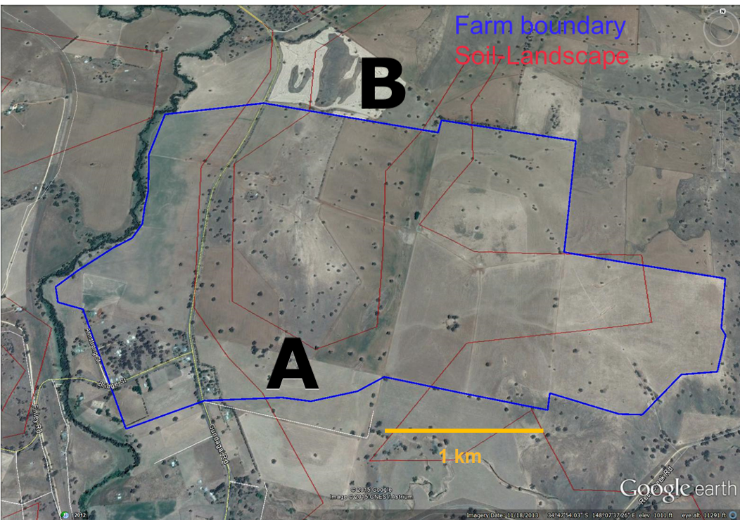
Land type A covers 62% of the area, land type B covers 38%
They sample randomly within each land type
For comparison, assume the same 7 locations happen to be selected

Random sampling on a landscape

import { samplingWidget } from "../../assets/js/sampling-widget.js"
samplingWidget({
  split: 0.62,
  labelA: "Land type A",
  labelB: "Land type B",
  nStart: 7,
  nMax: 30
})

With two distinct land types, how do we guarantee both are represented in our sample?

Simple Stratified random sampling

Stratified random sampling

3 steps

Divide the population into homogeneous subgroups (strata).
Sample from each stratum using simple random sampling.
Pool (combine) the estimates from each stratum to get an overall population estimate.

Example

If studying plant biodiversity in a national park:

Divide the park into strata (e.g. forest, grassland, wetland)
Take random samples within each habitat type
Combine data to estimate overall biodiversity, weighting by each habitat’s area

Strata rules

Strata are…

Mutually exclusive and collectively exhaustive: every unit belongs to exactly one stratum, with no overlaps and nothing left out
Homogeneous: units within a stratum should be more similar to each other than to the population as a whole
All sampled: every stratum must be represented

Advantages

Stratified random sampling addresses three problems at once:

Bias: every stratum is sampled, so the sample is representative of the population
Accuracy: each stratum is represented by a minimum number of units
Insight: we can compare strata and make inferences about subgroups

Does this make simple random sampling obsolete?

No. With large enough samples, the two methods converge. Simple random sampling is still a good default when strata are unknown or the population is fairly homogeneous.

Calculating stratified estimates

The workflow

Once we have our stratified sample, the calculations follow the same logic as simple random sampling, but each step must account for the stratified design.

Pooled mean (\(\bar{x}_{s}\)): weight each stratum mean by the stratum’s share of the population
Pooled standard error: \(SE(\bar{x}_{s}) = \sqrt{\sum w_i^2 \times \frac{s_i^2}{n_i}}\)
t-critical value: based on \(df = n - L\) and \(\alpha = 0.05\)
Confidence interval: \(\bar{x}_{s} \pm t_{n-L} \times SE(\bar{x}_{s})\)

Accounting for strata using “weight”

Each stratum contributes to the overall estimate in proportion to its size in the population.
Most of the time, we use the stratum’s share of the total area (or population) as the weight.
The overall population estimate is the sum of the weighted estimates from each stratum.

Soil carbon: setting up the data

The farmer collects the same 7 measurements as before. This time, each value is assigned to its land type:

landA <- c(90, 78, 86, 71)  # stratum A samples (62% of the area)
landB <- c(48, 56, 42)      # stratum B samples (38% of the area)

Pooled mean \(\bar x_{s}\)

The pooled mean is our best estimate of the overall population mean, taking into account the different stratum sizes.

\[\bar{x}_{s} = \sum_{i=1}^L \bar{x}_i \times w_i\]

We calculate the mean for each stratum (\(\bar{x}_i\)), multiply by its weight (\(w_i\)), and add them together.

Calculating pooled mean: soil carbon example

We first define the weights \(w_i\) for each stratum based on their area:

weight <- c(0.62, 0.38)  # 62% of area is land type A, 38% is land type B

Then we calculate the weighted mean:

weighted_mean <- mean(landA) * weight[1] + mean(landB) * weight[2]
weighted_mean

[1] 68.86833

Pooled standard error of the mean \(SE(\bar x_{s})\)

\[SE(\bar x_{s}) = \sqrt{\color{blue}{{\sum_{i=1}^L w_i^2}} \times \frac{s_i^2}{n_i}}\]

What is different from simple random sampling?

Instead of a single variance term, we sum the weighted variances from each stratum
The \(\color{blue}{w_i^2}\) term accounts for the relative size of each stratum
Each stratum contributes its own variance (\(s_i^2\)) and sample size (\(n_i\))

It is not as complicated as it sounds…

import { stratifiedStepsWidget } from "../../assets/js/sampling-widget.js"
stratifiedStepsWidget()

\(t\)-critical value

Degrees of freedom \(df\)

\[df = n - L\]

where \(n\) is the total number of samples and \(L\) is the number of strata.

For stratified sampling, we lose one degree of freedom for each stratum mean we estimate
Example: 12 samples across 3 strata gives \(df = 12 - 3 = 9\)

In R

df <- length(landA) + length(landB) - 2
t_crit <- qt(0.975, df)
t_crit

[1] 2.570582

Putting it all together in R

varA <- var(landA) / length(landA)  # variance of the mean for A
varB <- var(landB) / length(landB)  # variance of the mean for B
weighted_var <- weight[1]^2 * varA + weight[2]^2 * varB
weighted_se <- sqrt(weighted_var)
ci <- c(
  L95 = weighted_mean - t_crit * weighted_se,
  u95 = weighted_mean + t_crit * weighted_se
)
ci

     L95      u95 
61.04864 76.68803

The payoff

Simple random vs. stratified random sampling

The farmer sampled the same 7 locations using a stratified design. How do the results compare to simple random sampling?

Code

library(tidyverse)
# Manually printing the results below as SRS data is in previous lecture
compare <- tibble(
  Design = c("Simple Random", "Stratified Random"),
  Mean = c(67.29, 68.87),
  `Var (mean)` = c(50.80, 9.25),
  L95 = c(49.85, 61.05),
  U95 = c(84.73, 76.69),
  df = c(6, 5))
knitr::kable(compare)

Design	Mean	Var (mean)	L95	U95	df
Simple Random	67.29	50.80	49.85	84.73	6
Stratified Random	68.87	9.25	61.05	76.69	5

Visual comparison of 95% confidence intervals

Code

ggplot(compare, aes(x = Design, y = Mean)) +
  geom_point(size = 3) +
  geom_errorbar(aes(ymin = L95, ymax = U95), width = 0.2, linewidth = 1) +
  labs(title = "95% Confidence Intervals by Sampling Design",
       y = "Soil Carbon (tonnes/ha)",
       x = "") +
  theme_minimal(base_size = 14)

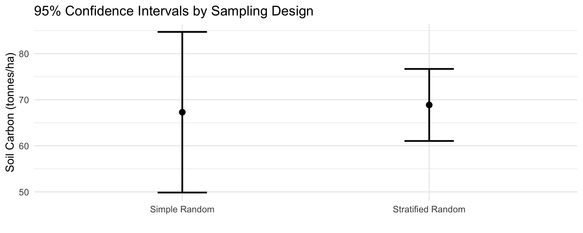
Key differences

Same locations, same measurements, different design
Stratified sampling gives a variance about 5 times smaller

Efficiency

How much more precise is stratified sampling?

\[\text{Efficiency} = \frac{\text{Variance of SRS}}{\text{Variance of Stratified}}\]

Efficiency > 1 means stratified sampling is more precise for the same sample size
An efficiency of 5 means you would need 5 times as many SRS samples to match the stratified precision

Efficiency (In R)

efficiency <- 50.80 / 9.25
efficiency

[1] 5.491892

How many SRS samples would we need for the same precision?

round(7 * efficiency, 0)

[1] 38

About 38 samples with SRS to match what 7 stratified samples achieved.

Tips on implementation

The hardest part is choosing good strata (e.g. soil types, elevation bands, land use)
Allocate samples in proportion to each stratum’s size
If one stratum is more variable, give it more samples

A year later…

Repeating the survey

The farmer now has a solid baseline. They know their soil carbon is around 69 t/ha with a tight confidence interval. A year passes. They introduce cover cropping and want to know: has soil carbon changed?

This is the second type of observational study we met in the first half, a monitoring study. Instead of estimating a single value, we are estimating change.

To answer this question, the farmer measures the same property again.

Same sites or new sites?

Key decision: how do we select sites for the second measurement?
1. Return to the same sites?
2. Select completely new sites?
This choice affects how we analyse the data

Change in mean \(\Delta \bar x\)

The difference between the means of the two sets of measurements.

\[\Delta \bar x = \bar x_2 - \bar x_1\]

where \(\bar x_2\) and \(\bar x_1\) are the means of the second and first set of measurements, respectively.

Why same sites give better estimates

Site 1 had 90 t/ha last year and 95 t/ha this year — a change of +5
We do not care that site 1 is naturally carbon-rich, only that it went up

Computing the difference at each site removes natural variation between sites
This is why paired sampling gives tighter confidence intervals

Paired vs independent sampling

Same sites → paired t-test
Different sites → two-sample t-test

Paired sampling is usually more precise
Each site is its own baseline, so natural differences drop out

Analysing change in R

R handles both approaches through t.test():

Same sites: t.test(after, before, paired = TRUE)
Different sites: t.test(after, before, paired = FALSE)

R connection

t.test() with paired = TRUE performs a paired t-test. You will use this in Lab 02 to analyse monitoring data.

The farmer’s journey

Today we followed one farmer through four problems, and each problem needed a new statistical tool:

“How do I choose where to sample?” → Simple random sampling
“How confident am I in the result?” → Confidence intervals
“Can I get a better estimate?” → Stratified random sampling
“Has anything changed?” → Monitoring and paired comparisons

Each concept built on the last. The same logic (estimate, quantify uncertainty, improve) runs through every sampling study you will encounter in this course.

Thanks!

Questions?

This presentation is based on the SOLES Quarto reveal.js template and is licensed under a Creative Commons Attribution 4.0 International License.