Lecture 03a – \(t\)-Tests

ENVX2001 Applied Statistical Methods

Januar Harianto

Apr 2026

The \(t\)-test (revision)

Introduction

One-sample \(t\)-test: compare a sample mean against a known value
Two-sample \(t\)-test: compare the means of two independent groups
Paired \(t\)-test: compare measurements taken on the same subjects (e.g. before and after)

Last week we learned about confidence intervals, which estimate the uncertainty of a parameter (e.g. a mean).

The \(t\)-test and the confidence interval are closely related. Both are derived from the same quantities, and this week we look at that connection more carefully.

Cattle

Two breeds of cattle, 12 and 15 samples. Are the breeds different in mean weight?

Code

cattle <- read.csv("data/cattle.csv") |>
  pivot_longer(cols = everything(), names_to = "breed", values_to = "weight") |>
  mutate(breed = as.factor(breed)) |>
  drop_na()

ggplot(cattle, aes(breed, weight)) +
  geom_boxplot() +
  labs(x = "Breed", y = "Weight (kg)") + 
  cowplot::theme_cowplot()

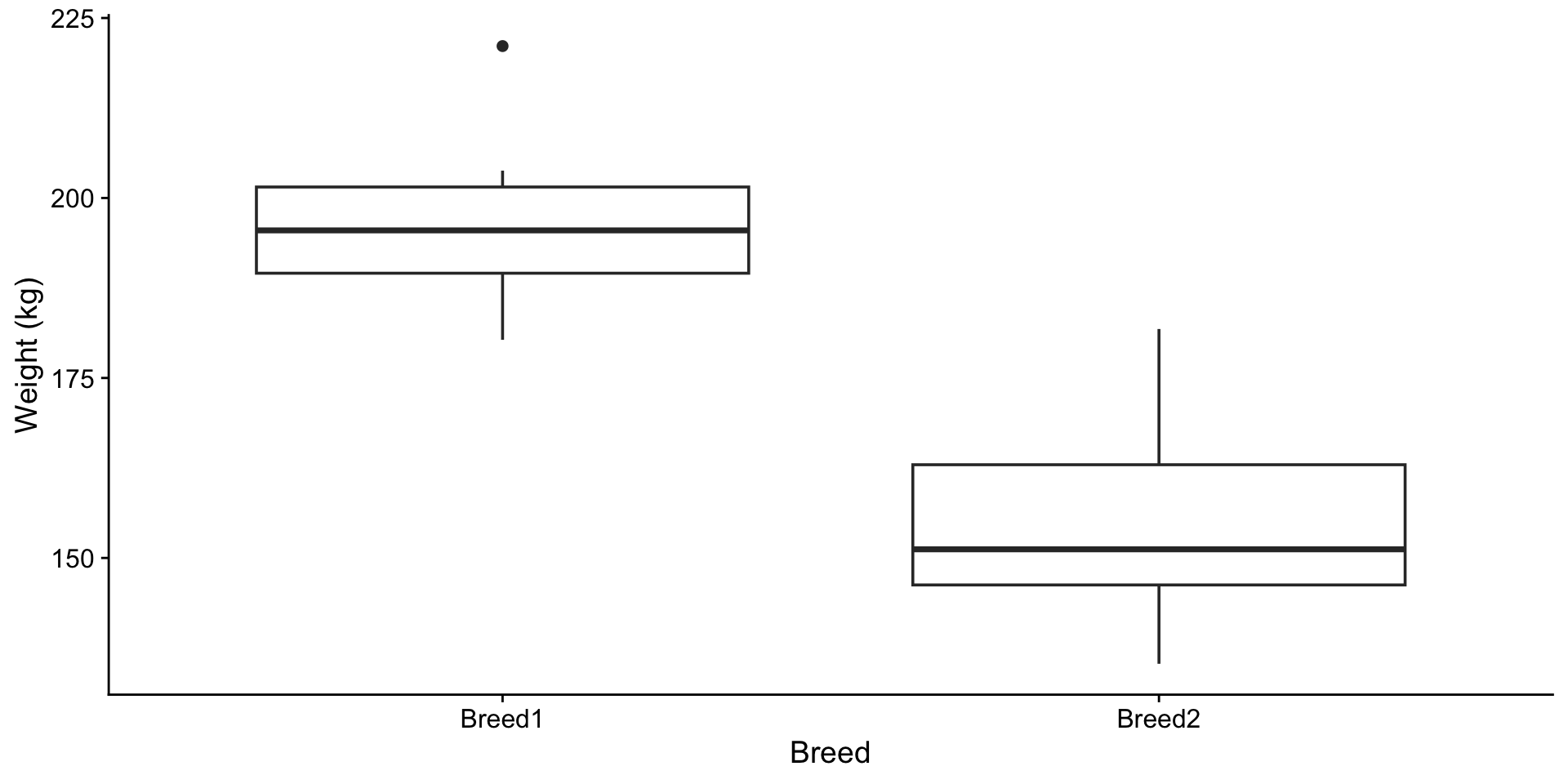
The boxplot suggests a difference. To test, you would run t.test() and check the p-value. What is the test actually computing?

From CIs to the \(t\)-test

The difference between two means

In the last lecture, we constructed confidence intervals for a single mean. The same principle extends to the difference between two means.

Estimate the difference: \(\bar{y}_1 - \bar{y}_2\)
Construct a 95% confidence interval around that estimate
Evaluate whether the interval includes zero

If the interval excludes zero: the means are significantly different at the 5% level
If the interval includes zero: the data are consistent with no difference

`t.test()` gives you both

Code

t.test(weight ~ breed, data = cattle, var.equal = TRUE)


    Two Sample t-test

data:  weight by breed
t = 9.4624, df = 25, p-value = 9.663e-10
alternative hypothesis: true difference in means between group Breed1 and group Breed2 is not equal to 0
95 percent confidence interval:
 33.23011 51.71989
sample estimates:
mean in group Breed1 mean in group Breed2 
             196.175              153.700

The output reports two quantities:

A p-value (probability of observing a result this extreme if the null hypothesis were true)
A 95% confidence interval for the difference between the two means

These always agree. If the CI excludes zero, the p-value is below 0.05, and vice versa. The \(t\)-statistic measures how far the observed difference is from zero, relative to its standard error.

Exploring the confidence interval

import { ciDifferenceWidget } from "../../assets/js/ttest-widget.js"
ciDifferenceWidget()

Increasing the difference between means moves the CI away from zero
Decreasing variability narrows the CI
When the interval excludes zero, the means are significantly different

The CI for a difference

In the last lecture, we built a 95% CI for a single mean:

\[\bar{y} \pm t^* \times SE\]

For the difference between two means, the same structure applies:

\[(\bar{y}_1 - \bar{y}_2) \pm t^* \times SE(\bar{y}_1 - \bar{y}_2)\]

If this interval excludes zero, the groups differ significantly.

The \(t\)-statistic

We can rearrange the CI formula to isolate a single number that captures both the difference and the variability:

\[t = \frac{\bar{y}_1 - \bar{y}_2}{SE(\bar{y}_1 - \bar{y}_2)}\]

The \(t\)-statistic counts how many standard errors the observed difference is from zero.

For the cattle data: \(t = 42.5 / 4.5 = 9.46\). The observed difference is over nine standard errors from zero.

From the \(t\)-statistic to the p-value

We have a \(t\)-statistic. The p-value answers: if there were truly no difference between the breeds, how often would we see a value of \(|t|\) this large or larger?

A small p-value means the observed difference is hard to explain by chance alone
A large p-value means the observed difference is consistent with random variation

The 95% CI and the p-value always agree. If the 95% CI excludes zero, the p-value is below 0.05, and vice versa.

Exploring the p-value

import { pvalueExplorerWidget } from "../../assets/js/ttest-widget.js"
pvalueExplorerWidget()

The shaded area under both tails is the p-value
As the \(t\)-statistic moves further from zero, the p-value decreases
At low degrees of freedom the tails are heavier, but the shape approaches the normal as df increases

The hypothesis testing workflow

Step 1: State what we are testing

Null hypothesis: \(H_0: \mu_1 = \mu_2\) (no difference in mean weight between breeds)
Alternative hypothesis: \(H_1: \mu_1 \neq \mu_2\) (means differ)
This is a two-tailed test: we are looking for a difference in either direction (Breed 1 heavier or lighter than Breed 2), not just one

Model equation: \(y_{ij} = \mu_i + \varepsilon_{ij}\)

Each observation is the group mean plus random error. The hypothesis asks whether \(\mu_1\) and \(\mu_2\) are equal.

Step 2a: Equal variances

The \(t\)-test assumes both groups have similar variability. If they do not, then the test is unreliable because the pooled estimate of variance will not represent either group well.

Rule of thumb: the ratio of the larger SD to the smaller SD should be below 2.0

Code

cattle_summary <- cattle |>
  group_by(breed) |>
  summarise(n = n(), mean_wt = mean(weight), sd_wt = sd(weight))

cattle_summary

# A tibble: 2 × 4
  breed      n mean_wt sd_wt
  <fct>  <int>   <dbl> <dbl>
1 Breed1    12    196.  10.6
2 Breed2    15    154.  12.3

Code

max(cattle_summary$sd_wt) / min(cattle_summary$sd_wt)

[1] 1.158756

Step 2b: Normality

The \(t\)-test assumes the data in each group follow a normal distribution. With small samples, departures from normality (strong skew, heavy tails, outliers) can distort the p-value and confidence interval. Check each group separately.

Code

shapiro.test(cattle$weight[cattle$breed == "Breed1"])


    Shapiro-Wilk normality test

data:  cattle$weight[cattle$breed == "Breed1"]
W = 0.94084, p-value = 0.5091

Code

shapiro.test(cattle$weight[cattle$breed == "Breed2"])


    Shapiro-Wilk normality test

data:  cattle$weight[cattle$breed == "Breed2"]
W = 0.94636, p-value = 0.4691

Step 2b: Normality (QQ plots)

Code

qqnorm(cattle$weight[cattle$breed == "Breed1"], main = "Breed 1")
qqline(cattle$weight[cattle$breed == "Breed1"])
qqnorm(cattle$weight[cattle$breed == "Breed2"], main = "Breed 2")
qqline(cattle$weight[cattle$breed == "Breed2"])

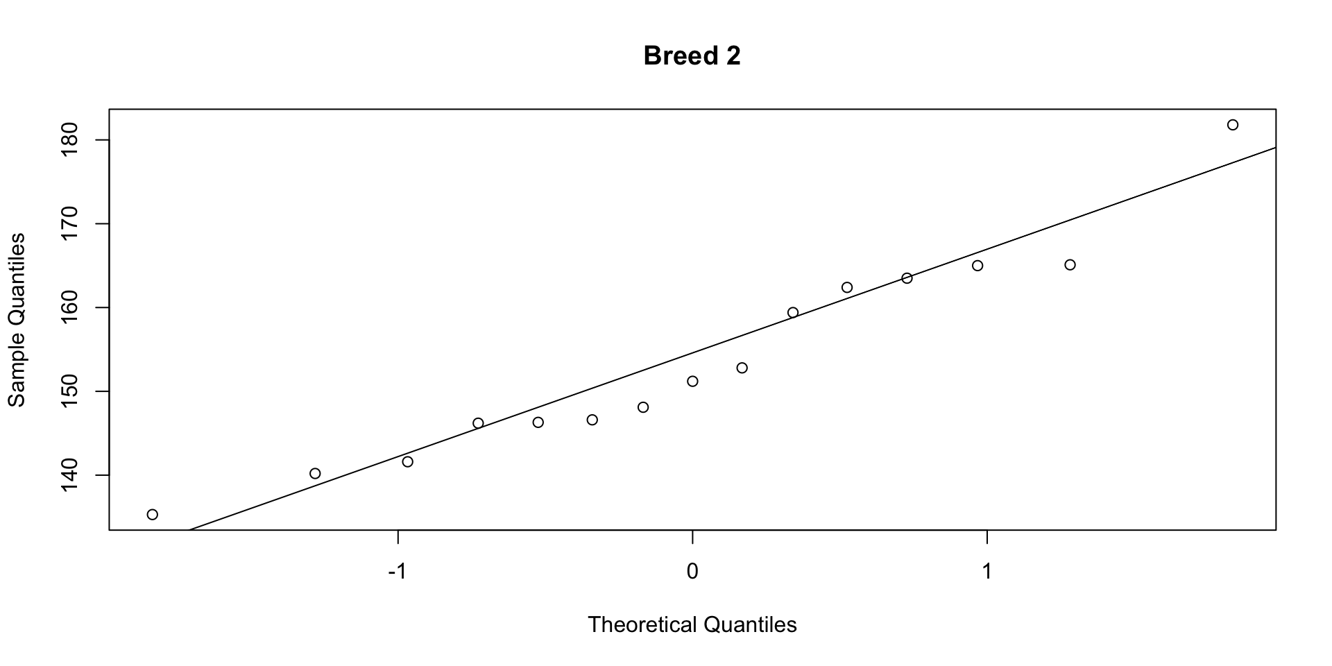
If points fall close to the line, the data are approximately normal. Both groups pass the Shapiro-Wilk test (\(p > 0.05\)) and the QQ plots show no strong departures.

Step 2c: Independence

Observations should not influence each other. This is a property of the study design, not something we test statistically.

Each animal is measured once
The weight of one animal does not affect the weight of another
If the same animals were measured before and after a treatment, observations would not be independent (use a paired \(t\)-test instead)

Step 3: Run the test and interpret

t.test(weight ~ breed, data = cattle, var.equal = TRUE)


    Two Sample t-test

data:  weight by breed
t = 9.4624, df = 25, p-value = 9.663e-10
alternative hypothesis: true difference in means between group Breed1 and group Breed2 is not equal to 0
95 percent confidence interval:
 33.23011 51.71989
sample estimates:
mean in group Breed1 mean in group Breed2 
             196.175              153.700

The \(t\)-statistic, degrees of freedom (\(n_1 + n_2 - 2\)), and p-value are reported together
var.equal = TRUE performs the pooled (Student’s) \(t\)-test, which assumes equal variances

A p-value of 0.03 does not mean there is a 3% chance the null hypothesis is true. It means: if there were truly no difference, we would observe a result this extreme about 3% of the time.

HATPC

Notice the five steps we just followed:

Hypotheses: state the null and alternative
Assumptions: check equal variances, normality, independence
Test: run the appropriate test
P-value: interpret the result
Conclusion: state the finding in context

We will use this framework throughout the semester, starting with ANOVA in the next lecture.

What if assumptions are not met?

Unequal variances: use Welch’s \(t\)-test (the default in R when var.equal = FALSE)
Non-normality: if \(N > 30\), the Central Limit Theorem provides reasonable coverage
Non-independence: consider a paired \(t\)-test (e.g. before and after measurements on the same subjects)

Summary

Key points

The two-sample \(t\)-test compares means of two independent groups
The \(t\)-test and the CI for the difference are two views of the same calculation
Check the three assumptions (equal variances, normality, independence) before running any test
Follow HATPC as a structured process for hypothesis testing

In Lab 03, you will practise this workflow with t.test() and diagnostic plots.

Next: what if we have more than two groups? We need ANOVA.

15 minute break

This presentation is based on the SOLES Quarto reveal.js template and is licensed under a Creative Commons Attribution 4.0 International License.

Lecture 03a – \(t\)-Tests

The \(t\)-test (revision)

Introduction

Cattle

From CIs to the \(t\)-test

The difference between two means

t.test() gives you both

Exploring the confidence interval

The CI for a difference

The \(t\)-statistic

From the \(t\)-statistic to the p-value

Exploring the p-value

The hypothesis testing workflow

Step 1: State what we are testing

Step 2a: Equal variances

Step 2b: Normality

Step 2b: Normality (QQ plots)

Step 2c: Independence

Step 3: Run the test and interpret

HATPC

What if assumptions are not met?

Summary

Key points

15 minute break

`t.test()` gives you both