Lecture 03b – One-way ANOVA

ENVX2001 Applied Statistical Methods

Januar Harianto

Apr 2026

From \(t\)-tests to ANOVA

From two groups to four

Before the break we compared two cattle breeds. But what if there were four breeds instead of two?

  • Can we still use \(t\)-tests? Yes, but we would need to test every pair
  • With 4 groups that is \(\binom{4}{2} = 6\) comparisons: 1 vs 2, 1 vs 3, 1 vs 4, 2 vs 3, 2 vs 4, 3 vs 4

The problem: every test carries a risk of a Type I error (a false positive).

  • We set \(\alpha = 0.05\), so each comparison has a 5% chance of rejecting \(H_0\) when it is actually true
  • Six tests means six chances to get it wrong

The multiple comparisons problem

With 6 groups there are \(\binom{6}{2} = 15\) pairwise comparisons. The probability that none produce a false positive is \(0.95^{15}\), so:

\[P(\text{at least one false positive}) = 1 - 0.95^{15} = 53.7\%\]

Groups Pairwise tests P(at least one false positive)
2 1 5.0%
4 6 26.5%
6 15 53.7%
8 28 76.2%
10 45 90.1%
  • With 10 groups, a false positive is almost guaranteed
  • We need a method that tests all groups at once

Chick feeding

The experiment

We need a method that handles more than two groups. Consider a new experiment:

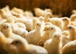
  • 20 chicks are randomly assigned to one of 4 diets
  • 5 replicates per diet
  • Response: weight gain (g)
chicks <- read.csv("data/chicks.csv") |>
  pivot_longer(
    starts_with("Diet"), names_to = "diet", values_to = "weight"
  ) |>
  mutate(diet = as.factor(diet))

Are there differences?

Code
ggplot(chicks, aes(diet, weight)) +
  geom_boxplot() +
  labs(x = "Diet", y = "Weight gain (g)") +
  cowplot::theme_cowplot()

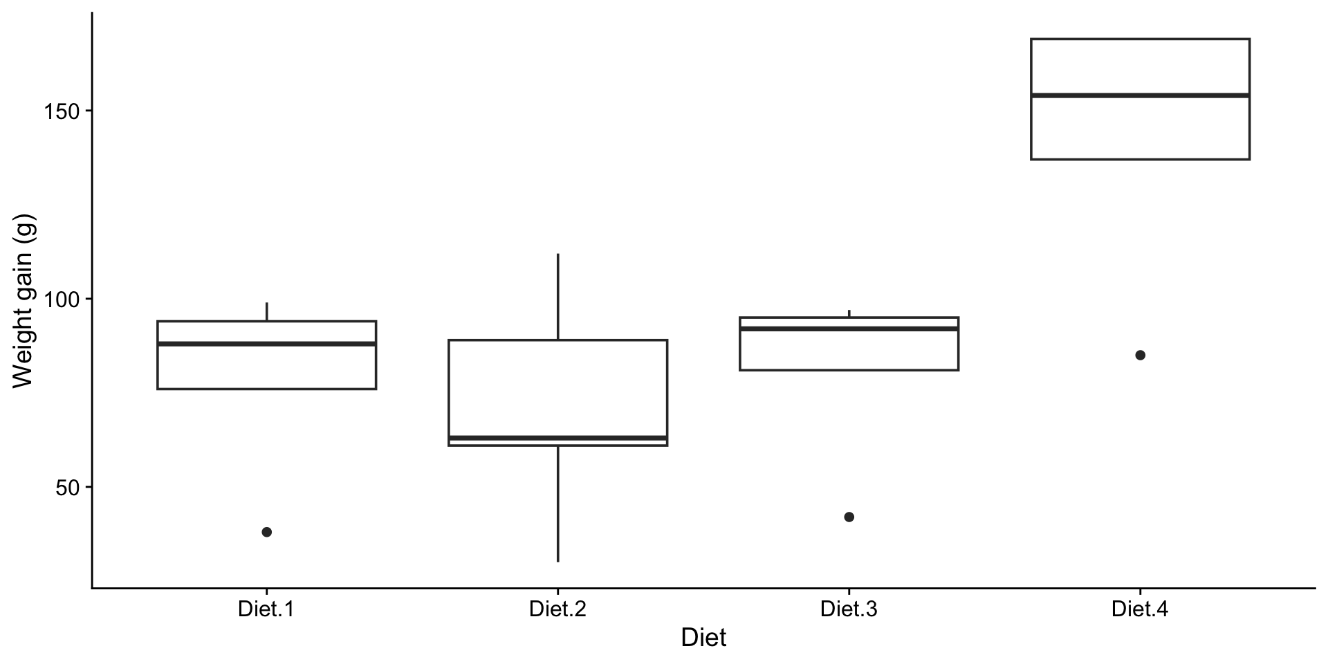
What do the boxplots suggest?

Terminology

Term Meaning In this experiment
Factor Categorical variable being tested Diet
Levels Categories within a factor Diet 1, Diet 2, Diet 3, Diet 4
Replicates Observations per level \(r = 5\)

This is a one-way ANOVA because there is only one factor. What is ANOVA?

HATPC for Analysis of Variance

H: Hypotheses

In the \(t\)-test we asked whether two means were equal. ANOVA extends this to any number of groups.

  • Null hypothesis: \(H_0: \mu_1 = \mu_2 = \mu_3 = \mu_4\)
  • Alternative hypothesis: \(H_1:\) not all \(\mu_i\) are equal

The alternative does not say all means differ. It says at least two do.

Model equation:

\[y_{ij} = \mu_i + \varepsilon_{ij}\]

where \(i = 1, \ldots, t\) treatments and \(j = 1, \ldots, n_i\) replicates. The same structure as the \(t\)-test model, but \(i\) now ranges over more than two groups.

A: Assumptions

The same three assumptions from the \(t\)-test apply here. We fit the model first, then check.

model <- aov(weight ~ diet, data = chicks)

Normality (Shapiro-Wilk on residuals):

Code
shapiro.test(residuals(model))

    Shapiro-Wilk normality test

data:  residuals(model)
W = 0.90961, p-value = 0.06265

\(p > 0.05\): no evidence against normality.

Equal variances (Bartlett’s test):

Code
bartlett.test(weight ~ diet, data = chicks)

    Bartlett test of homogeneity of variances

data:  weight by diet
Bartlett's K-squared = 0.85164, df = 3, p-value = 0.8371

\(p > 0.05\): variances are similar across groups.

A: Residual diagnostics

Code
qqnorm(residuals(model), main = "Normal QQ plot")
qqline(residuals(model))
plot(fitted(model), residuals(model),
     xlab = "Fitted values", ylab = "Residuals",
     main = "Residuals vs Fitted")
abline(h = 0, lty = 2)

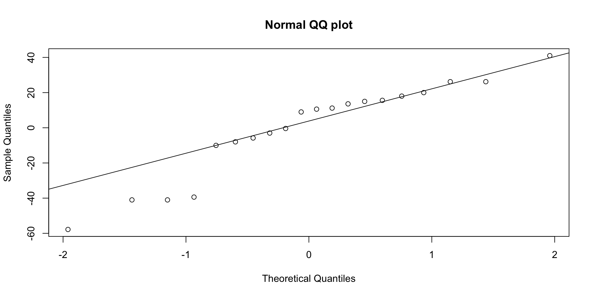
  • QQ plot: points follow the line, supporting normality
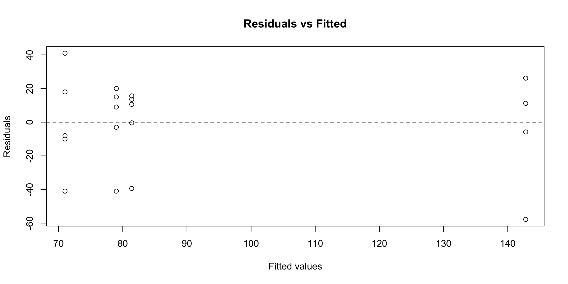
  • Residuals vs fitted: no fan shape, supporting equal variances
  • Independence holds by design: each chick is measured once

A: A shortcut for next time

R can produce all standard diagnostic plots at once:

plot(model)

We will explore these plots in detail next week. For now, the Shapiro-Wilk and Bartlett’s tests are sufficient.

T: The ANOVA idea

  • How does ANOVA decide whether these four diets differ?
  • If diets matter, differences between groups should be large relative to variation within groups
Code
overall_mean <- mean(chicks$weight)
group_means <- chicks |>
  group_by(diet) |>
  summarise(mean_wt = mean(weight))

p1 <- ggplot(chicks, aes(diet, weight)) +
  geom_point(size = 3, alpha = 0.6) +
  geom_hline(data = group_means, aes(yintercept = mean_wt),
    linetype = "dashed", colour = "#e64626", linewidth = 0.8) +
  labs(title = "Four group means", x = "Diet", y = "Weight gain (g)") +
  cowplot::theme_cowplot()

p2 <- ggplot(chicks, aes(diet, weight)) +
  geom_point(size = 3, alpha = 0.6) +
  geom_hline(yintercept = overall_mean, colour = "#e64626",
    linewidth = 0.8, linetype = "dashed") +
  labs(title = "One overall mean", x = "Diet", y = "Weight gain (g)") +
  cowplot::theme_cowplot()

library(patchwork)
p1 + p2

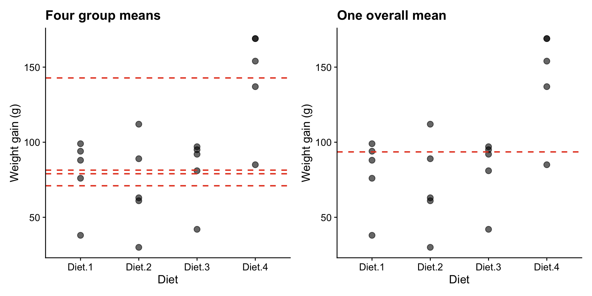
Do four separate means (left) explain the data better than a single overall mean (right)?

Two sources of variation

ANOVA splits the total variation in the data into two parts:

  • Between-group variation (orange): how far each group mean is from the overall mean. If diets matter, this should be large.
  • Within-group variation (black): how much individual observations scatter around their own group mean. This is random noise.

ANOVA compares these two quantities. If between-group variation is large relative to within-group variation, we have evidence that the groups genuinely differ.

Variance partitioning

The F ratio

\[F = \frac{MS_{\text{trt}}}{MS_{\text{res}}}\]

  • \(F\) compares variation due to group differences against random noise
  • MS (mean square) is based on squared deviations: squaring prevents positive and negative differences from cancelling out
  • When \(H_0\) is true (all groups equal), \(F \approx 1\)
  • When groups genuinely differ, \(F \gg 1\)

For two groups, ANOVA gives the same answer as the \(t\)-test:

\[F = t^2\]

ANOVA extends the \(t\)-test to any number of groups.

T: The ANOVA table

Source df SS MS F
Treatment \(t - 1\) \(SS_{\text{trt}}\) \(SS_{\text{trt}} / (t-1)\) \(MS_{\text{trt}} / MS_{\text{res}}\)
Residual \(N - t\) \(SS_{\text{res}}\) \(SS_{\text{res}} / (N-t)\)
Total \(N - 1\) \(SS_{\text{total}}\)
model <- aov(weight ~ diet, data = chicks)
summary(model)
            Df Sum Sq Mean Sq F value Pr(>F)   
diet         3  16467    5489   6.647  0.004 **
Residuals   16  13212     826                  
---
Signif. codes:  0 '***' 0.001 '**' 0.01 '*' 0.05 '.' 0.1 ' ' 1

P: Interpret

  • diet row: variation explained by the four diets (\(df = 3\), since 4 groups minus 1)
  • Residuals row: leftover variation (\(df = 16\), since 20 observations minus 4 groups)
  • \(F = 6.65\): the treatment variance is 6.65 times larger than the residual variance
  • \(p = 0.004\): below 0.05, so we reject \(H_0\)

How much variability is explained?

\[\frac{SS_{\text{treatment}}}{SS_{\text{total}}} = \frac{1.6467\times 10^{4}}{2.9679\times 10^{4}} = 55.5\%\]

The diets explain about 55% of the total variability in chick weight gain.

C: Conclusion

Source df SS MS F p
Diet 3 1.6467^{4} 5489 6.65 0.004
Residual 16 1.3212^{4} 825.8

There are significant differences in mean weight gain among the four diets (\(F_{3,16} = 6.65\), \(p = 0.004\)).

But ANOVA only tells us that groups differ, not which ones. To identify specific differences, we need post-hoc analysis.

Post-hoc

Why post-hoc?

\(H_1\) says “not all means are equal,” but not which ones differ.

  • ANOVA tells us the four diet means are not all the same
  • It does not tell us whether Diet 1 differs from Diet 2, or Diet 3 from Diet 4
  • We cannot run separate \(t\)-tests (the multiple comparisons problem from the first slide)
  • We need a method that compares pairs while controlling the overall error rate

Post-hoc and confidence intervals

Before the break we used a confidence interval for the difference between two cattle breeds. Post-hoc methods apply the same logic to every pair of groups.

  • For each pair, construct a CI for the difference in means
  • If the CI excludes zero, those two groups differ significantly
  • If the CI includes zero, we cannot conclude they differ

The key difference from running separate \(t\)-tests: post-hoc methods widen the CIs to account for multiple comparisons, keeping the overall false positive rate at 5%.

We will cover specific post-hoc methods (Tukey, Bonferroni) in detail next week.

Estimated marginal means

Before the break we used CIs to compare two cattle breeds. The same idea extends to multiple groups. emmeans estimates the mean and standard error for each group from the model.

library(emmeans)
emm <- emmeans(model, "diet")
emm
 diet   emmean   SE df lower.CL upper.CL
 Diet.1   79.0 12.9 16     51.8    106.2
 Diet.2   71.0 12.9 16     43.8     98.2
 Diet.3   81.4 12.9 16     54.2    108.6
 Diet.4  142.8 12.9 16    115.6    170.0

Confidence level used: 0.95 

Pairwise comparisons

To find which pairs differ, we construct a CI for the difference between every pair of means.

confint(pairs(emm))
 contrast        estimate   SE df lower.CL upper.CL
 Diet.1 - Diet.2      8.0 18.2 16    -44.0     60.0
 Diet.1 - Diet.3     -2.4 18.2 16    -54.4     49.6
 Diet.1 - Diet.4    -63.8 18.2 16   -115.8    -11.8
 Diet.2 - Diet.3    -10.4 18.2 16    -62.4     41.6
 Diet.2 - Diet.4    -71.8 18.2 16   -123.8    -19.8
 Diet.3 - Diet.4    -61.4 18.2 16   -113.4     -9.4

Confidence level used: 0.95 
Conf-level adjustment: tukey method for comparing a family of 4 estimates 
  • Each row is one pairwise comparison (e.g. Diet1 - Diet2)
  • The lower.CL and upper.CL columns are the 95% CI for the difference
  • If the CI excludes zero, those two diets differ significantly

Visualising the comparisons

plot(emm, comparisons = TRUE) +
  labs(x = "Weight gain (g)", y = "Diet")
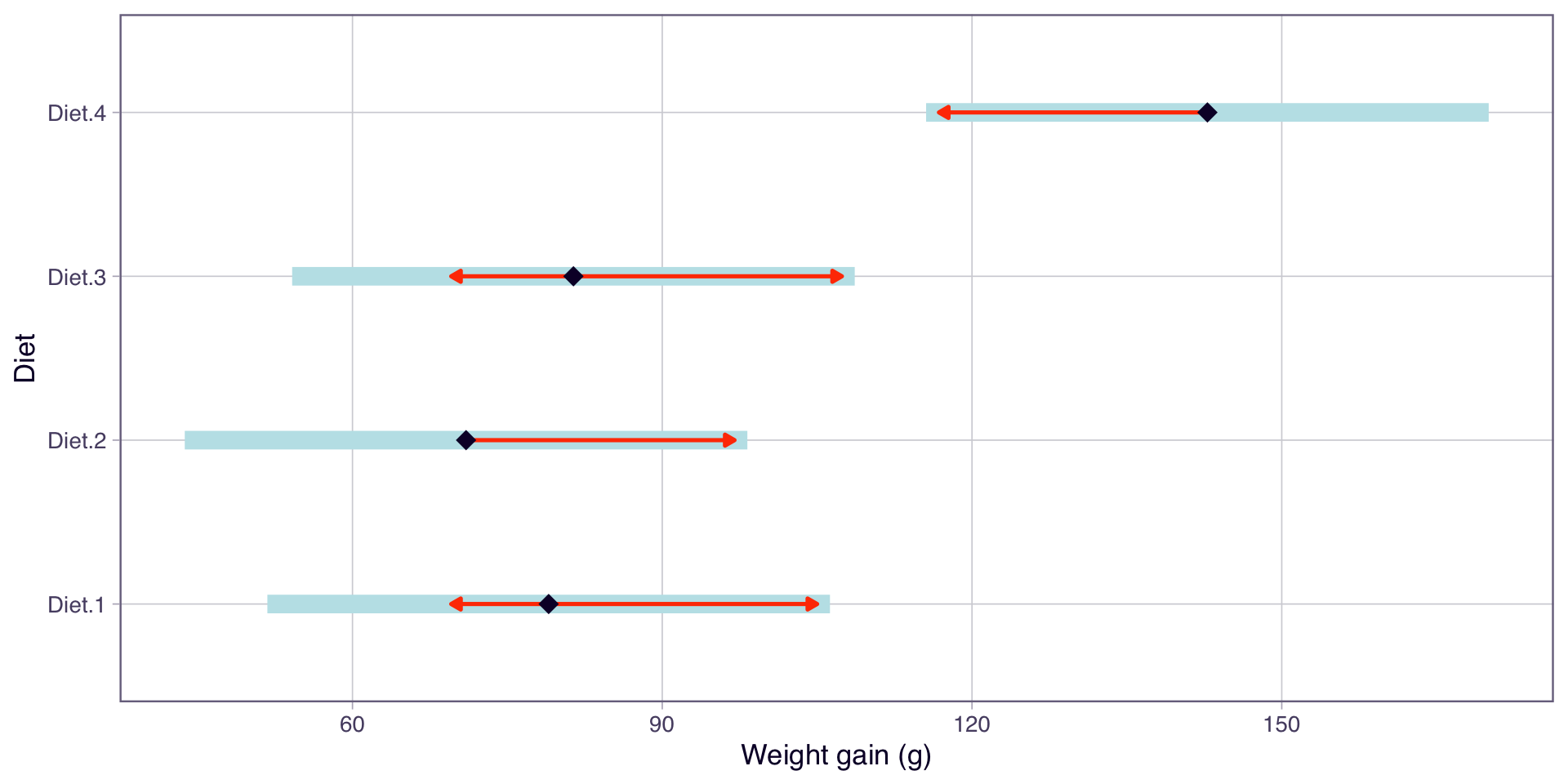
  • Each point is the estimated mean for that diet
  • The arrows represent comparison intervals (adjusted CIs)
  • Groups with overlapping arrows are not significantly different
  • We will cover post-hoc methods in more detail next week

Summary

Key points

  • ANOVA extends the \(t\)-test to more than two groups (\(F = t^2\) for two groups)
  • Multiple pairwise \(t\)-tests inflate the false positive rate. ANOVA tests all groups at once
  • The F ratio compares between-group variation to within-group variation
  • Post-hoc methods construct CIs for pairwise differences to identify which groups differ

In Lab 03, you will fit your own ANOVA with aov() and explore group comparisons with emmeans. Next week: residual diagnostics and post-hoc methods.

Thanks!

Questions?

This presentation is based on the SOLES Quarto reveal.js template and is licensed under a Creative Commons Attribution 4.0 International License.