Welcome

In this tutorial you will compute confidence intervals from a real dataset and see what happens when you ignore group structure in your sample.

You will learn how to:

Load a real dataset and compute a confidence interval using t.test().
Understand what a confidence interval tells you (and what it does not).
See why accounting for group structure matters when estimating a population parameter.

The dataset for today comes from the DAAG package. The possum dataset contains measurements on 104 mountain brushtail possums (Trichosurus caninus) captured at seven sites across south-eastern Australia, from a study by Lindenmayer et al. (1995). Researchers captured possums at field sites in Victoria and in parts of Queensland and New South Wales, recording morphological measurements such as head length, skull width, tail length, and ear conch length.

library(DAAG)
data(possum)

If you have not installed DAAG before, run install.packages("DAAG") in the console first. You only need to do this once.

1 Confidence intervals

A confidence interval gives you a range of plausible values for something you cannot measure directly — like the true mean of a population. It tells you how precise your estimate is, based on the data you have.

Exercise 1: What confidence intervals tell us

Part A — Compute and interpret

Start by inspecting the dataset:

str(possum)

'data.frame':   104 obs. of  14 variables:
 $ case    : num  1 2 3 4 5 6 7 8 9 10 ...
 $ site    : num  1 1 1 1 1 1 1 1 1 1 ...
 $ Pop     : Factor w/ 2 levels "Vic","other": 1 1 1 1 1 1 1 1 1 1 ...
 $ sex     : Factor w/ 2 levels "f","m": 2 1 1 1 1 1 2 1 1 1 ...
 $ age     : num  8 6 6 6 2 1 2 6 9 6 ...
 $ hdlngth : num  94.1 92.5 94 93.2 91.5 93.1 95.3 94.8 93.4 91.8 ...
 $ skullw  : num  60.4 57.6 60 57.1 56.3 54.8 58.2 57.6 56.3 58 ...
 $ totlngth: num  89 91.5 95.5 92 85.5 90.5 89.5 91 91.5 89.5 ...
 $ taill   : num  36 36.5 39 38 36 35.5 36 37 37 37.5 ...
 $ footlgth: num  74.5 72.5 75.4 76.1 71 73.2 71.5 72.7 72.4 70.9 ...
 $ earconch: num  54.5 51.2 51.9 52.2 53.2 53.6 52 53.9 52.9 53.4 ...
 $ eye     : num  15.2 16 15.5 15.2 15.1 14.2 14.2 14.5 15.5 14.4 ...
 $ chest   : num  28 28.5 30 28 28.5 30 30 29 28 27.5 ...
 $ belly   : num  36 33 34 34 33 32 34.5 34 33 32 ...

There are 104 observations and 14 variables, including measurements of head length, skull width, and tail length. We will focus on head length.

Compute a 95% confidence interval for the mean head length:

t.test(possum$hdlngth)


    One Sample t-test

data:  possum$hdlngth
t = 264.28, df = 103, p-value < 2.2e-16
alternative hypothesis: true mean is not equal to 0
95 percent confidence interval:
 91.90796 93.29781
sample estimates:
mean of x 
 92.60288

The sample mean head length is 92.6 mm. The 95% confidence interval is approximately [91.9, 93.3].

What does this interval actually mean? If we repeated this study many times — catching a fresh group of 104 possums each time — about 95% of the intervals we compute would contain the true population mean.

You might think this means there is a 95% probability the true mean lies inside this particular interval. Not quite. The true mean is a fixed value — it is either inside the interval or it is not. We just do not know which.

So we are reasonably confident that the average head length of mountain brushtail possums in this region is somewhere between 91.9 and 93.3 mm.

The 95% refers to the long-run success rate of the method, not the probability for any single interval.

Part B — What affects the width?

What if we had measured fewer possums? Would our confidence interval change?

Draw a random sample of 10 possums and compute the confidence interval:

set.seed(2026)
samp10 <- sample(possum$hdlngth, 10)
t.test(samp10)


    One Sample t-test

data:  samp10
t = 74.625, df = 9, p-value = 7.048e-14
alternative hypothesis: true mean is not equal to 0
95 percent confidence interval:
 89.44386 95.03614
sample estimates:
mean of x 
    92.24

Now draw a sample of 50:

set.seed(2026)
samp50 <- sample(possum$hdlngth, 50)
t.test(samp50)


    One Sample t-test

data:  samp50
t = 181.77, df = 49, p-value < 2.2e-16
alternative hypothesis: true mean is not equal to 0
95 percent confidence interval:
 91.13518 93.17282
sample estimates:
mean of x 
   92.154

Compare the widths. With 10 possums the interval is roughly 5.6 mm wide. With 50 it narrows to about 2.0 mm. With all 104 it is only 1.4 mm. More data, narrower interval.

This happens because the standard error is SD / \sqrt{n}. As n increases, the standard error shrinks, and so does the confidence interval. This is what t.test() computes internally.

Try changing the seed or the sample size and re-running to see how your interval changes.

Checkpoint

You should be able to explain what a 95% confidence interval means in plain language and why a larger sample gives a narrower interval.

2 Sampling and group structure

So far we have treated all 104 possums as one group. But what happens when a population contains distinct subgroups?

Exercise 2: When groups matter

Part A — The pooled estimate

Compute a confidence interval for ear conch length across all possums:

t.test(possum$earconch)


    One Sample t-test

data:  possum$earconch
t = 119.44, df = 103, p-value < 2.2e-16
alternative hypothesis: true mean is not equal to 0
95 percent confidence interval:
 47.33160 48.92994
sample estimates:
mean of x 
 48.13077

This interval estimates the average ear conch length — the length of the outer ear opening — across all 104 possums. The mean is about 48.1 mm, with a 95% CI of roughly [47.3, 48.9].

But these possums come from two distinct populations: Victorian possums from sites in central and eastern Victoria, and possums from sites further north in New South Wales and Queensland.

Part B — Split by population

Compute separate confidence intervals for each population:

t.test(possum$earconch[possum$Pop == "Vic"])


    One Sample t-test

data:  possum$earconch[possum$Pop == "Vic"]
t = 153.2, df = 45, p-value < 2.2e-16
alternative hypothesis: true mean is not equal to 0
95 percent confidence interval:
 51.50087 52.87304
sample estimates:
mean of x 
 52.18696

t.test(possum$earconch[possum$Pop == "other"])


    One Sample t-test

data:  possum$earconch[possum$Pop == "other"]
t = 216.63, df = 57, p-value < 2.2e-16
alternative hypothesis: true mean is not equal to 0
95 percent confidence interval:
 44.49862 45.32896
sample estimates:
mean of x 
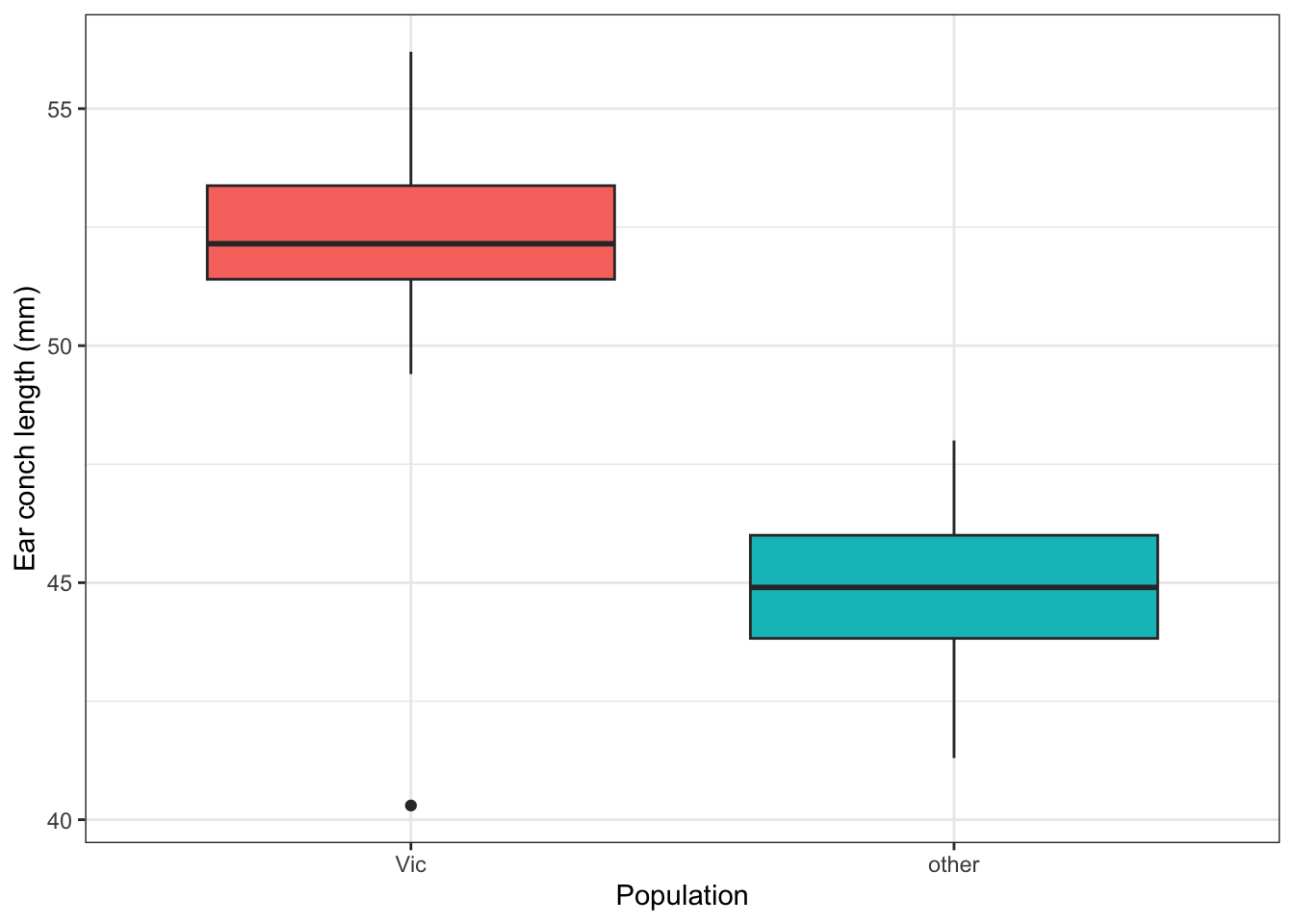
 44.91379

The Victorian possums have a mean ear conch length of about 52.2 mm. The other population averages about 44.9 mm — over 7 mm shorter. The pooled confidence interval of [47.3, 48.9] sits between the two groups. It does not describe either population well.

A boxplot makes the separation clear:

library(ggplot2)

ggplot(possum, aes(x = Pop, y = earconch, fill = Pop)) +
  geom_boxplot(show.legend = FALSE) +
  labs(x = "Population", y = "Ear conch length (mm)") +
  theme_bw()

Figure 1: Ear conch length by population

Part C — Connection to the lab

When a population has distinct subgroups, a single estimate can hide real differences. In the lab, you will learn stratified random sampling — a method that estimates each subgroup separately and then combines them into a single, more accurate overall estimate.

Checkpoint

You should be able to explain why computing a single confidence interval for a population with distinct subgroups can be misleading.

Wrap-up

In this tutorial you computed confidence intervals and saw why sample size and group structure both matter. You will use these ideas in the lab.