---
title: "Tutorial 04"
# reviewed-by: Aaron Greenville
format:
sandstone-html:
code-tools: true
---
```{r setup, include=FALSE}
knitr::opts_chunk$set(echo = TRUE)
```
## Welcome {.unnumbered}
In this week's lectures we covered how to check the assumptions of ANOVA using residual diagnostics, and how to determine which pairs of treatment means are significantly different using post-hoc tests. A solid understanding of these concepts is essential for conducting robust statistical analyses in R and before we move to more complex models in future weeks.
You will learn how to:
1. Assess whether a fitted ANOVA model meets its statistical assumptions using residuals.
2. Test the assumptions of normality and homogeneity of variances using graphical methods and statistical tests.
3. Identify which pair(s) of treatment means are significantly different using post-hoc tests.
4. Understand the trade-off between controlling the family-wise error rate and maintaining statistical power.
We will assume we have formed a hypothesis, designed an experiment, collected data and entered it into R. In our case we have chosen an ANOVA for our model and now need to do an assessment of model assumptions.
# Assessing ANOVA assumptions using residuals
## Exercise 1: Why use residuals {.unnumbered}
Residuals are the differences between the observed values and the values predicted by our statistical model. In the context of ANOVA, residuals help us assess how well our model fits the data.
Mathematically, the residual for each observation can be calculated as:
$$
\text{Residual} = \text{Observed Value} - \text{Predicted Value}
$$
Residuals have key advantages over raw data for testing assumptions and you will be required to use the residuals of your model to test the assumptions of ANOVA and regression from now on.
### Part A --- Synthetic data demonstration
::: {.column-margin}
This exercise illustrates why it is not ideal to test the normality assumption using all of the observations irrespective of the treatments or the size of dataset.
:::
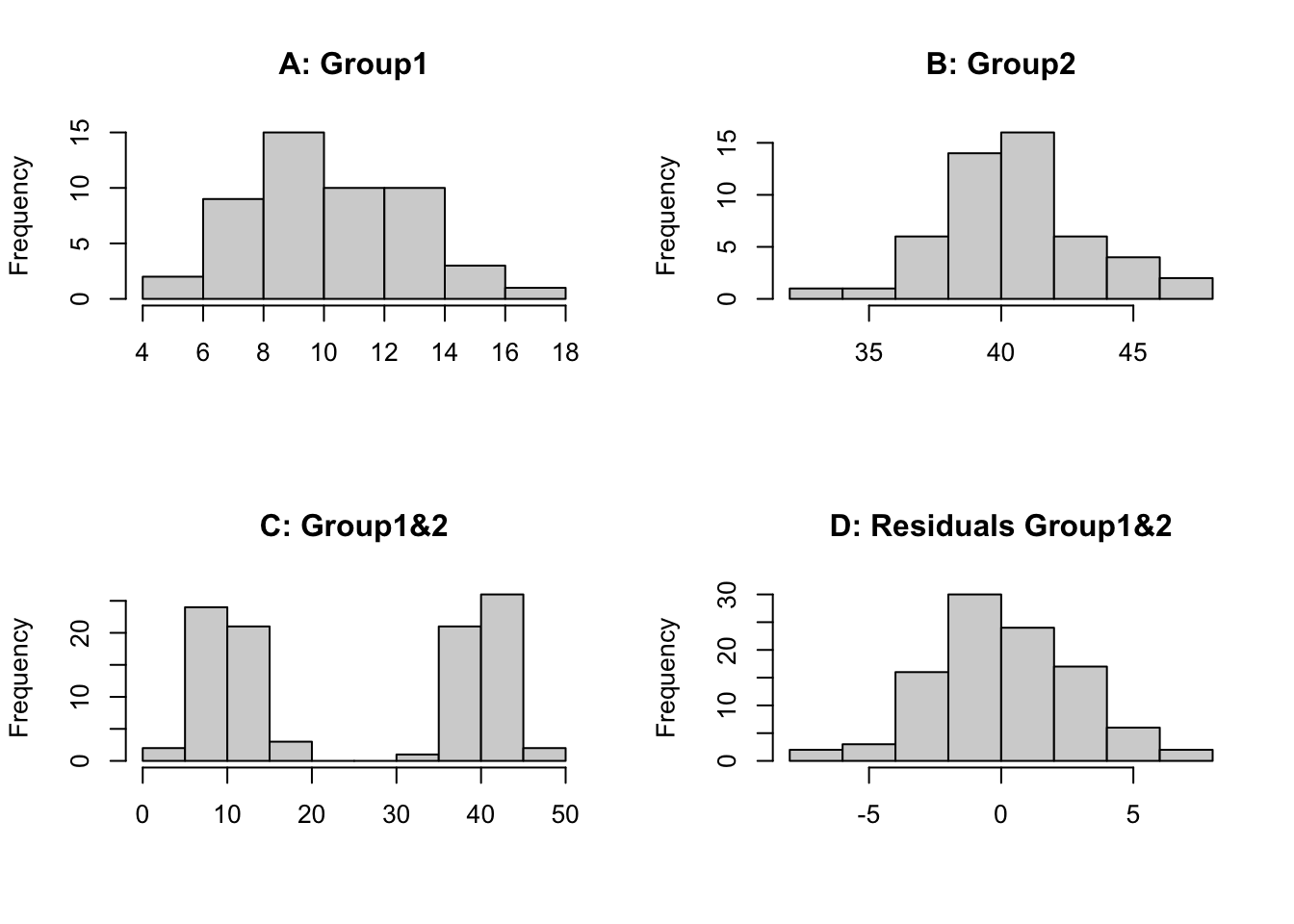
First we will create 2 synthetic datasets which we sample 50 times (`n=50`) from a normally distributed population. Both underlying populations have the same variation (`sd=3`) but have a different mean (`mean=10`, `mean=40`). We then plot the histograms for each individually, both groups combined and the combined residuals (observation minus group mean).
```{r}
set.seed(123)
group1 <- rnorm(n = 50, mean = 10, sd = 3)
group2 <- rnorm(n = 50, mean = 40, sd = 3)

par(mfrow = c(2, 2))
hist(group1, main = "A: Group1", xlab = "")
hist(group2, main = "B: Group2", xlab = "")
hist(c(group1, group2), main = "C: Group1&2", xlab = "")
hist(c(group1 - mean(group1), group2 - mean(group2)), main = "D: Residuals Group1&2", xlab = "")
par(mfrow = c(1, 1))
```
We can see that histogram of each group is normally distributed (A, B), however when we combine the data we have 2 distinct groupings centred on the mean of each group (C). Therefore, if we look at the raw data irrespective of the groups we **would not see a normally distributed dataset**. This is because the effect of individual treatments (or groups) is different so each observation is perturbed according to the treatment it receives or group it is in. If we examine the residuals (D), the treatment (or group) effects have been removed and we can then test if the data is normal or has constant variance. It requires fitting of a model to the data, in this case a 1-way ANOVA model. This is why we test the assumptions on the residuals. You could look at the distribution of each group separately but then for some experiments the replication is small so it is hard to assess normality, using residuals allows all of the observations to be pooled together.
### Part B --- Fitting ANOVA and extracting residuals
Now we will fit a one-way ANOVA model to the data and extract the residuals to test the assumptions of normality and homogeneity of variance.
```{r}
# Create a data frame
data <- data.frame(
value = c(group1, group2),
group = as.factor(rep(c("Group1", "Group2"), each = 50))
)
# Fit a one-way ANOVA model
anova_model <- aov(value ~ group, data = data)
# Extract residuals
residuals_anova <- residuals(anova_model)
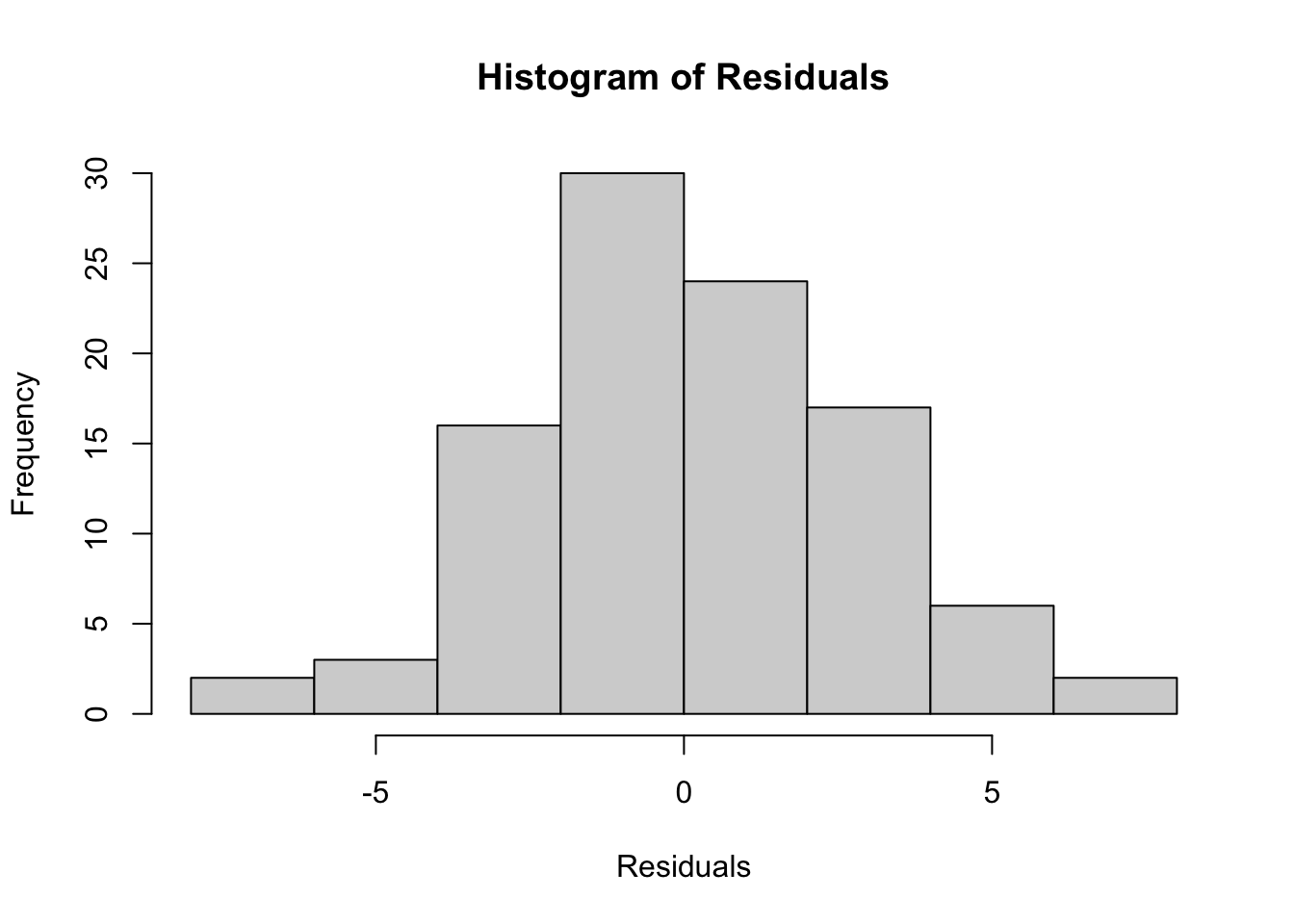
# Plot histogram of residuals
hist(residuals_anova, main = "Histogram of Residuals", xlab = "Residuals")
```
We can see that the histogram of the residuals appears to be normally distributed.
We can compare this to the histogram of the raw data (also plot C above).
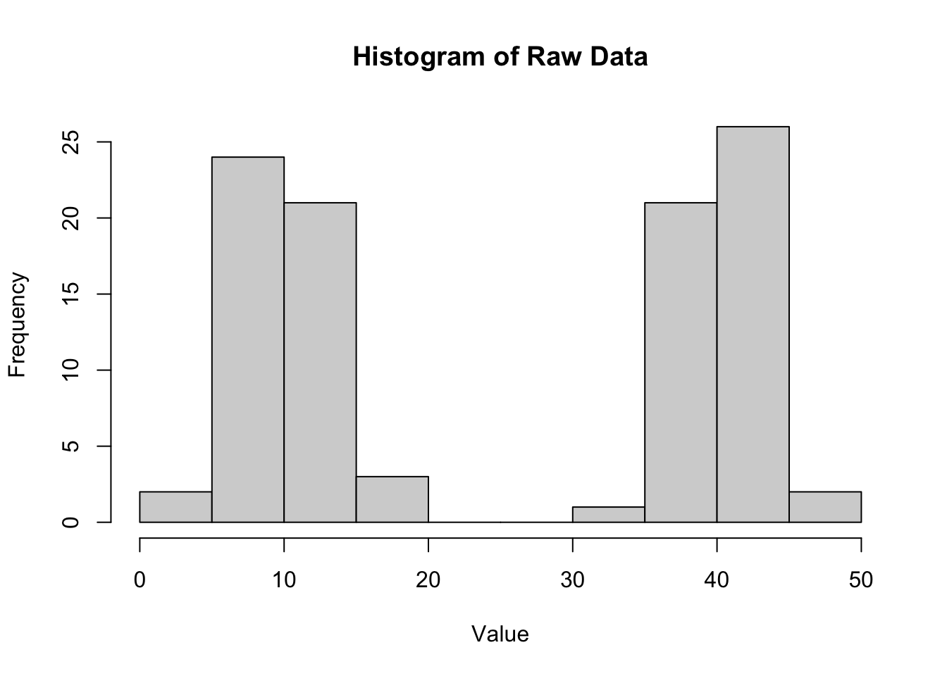
```{r}
# Plot histogram of raw data
hist(data$value, main = "Histogram of Raw Data", xlab = "Value")
```
The histogram of the raw data shows two distinct peaks corresponding to the two groups, indicating that the data is not normally distributed when considering all observations together. This highlights the importance of using residuals to assess normality in the context of ANOVA.
### Part C --- Q-Q plot
We can also create a Q-Q plot to further assess normality.
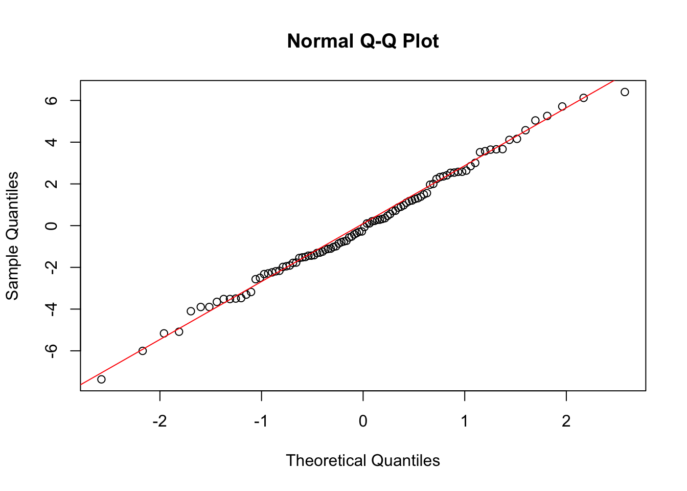
```{r}
# Q-Q plot of residuals
qqnorm(residuals_anova)
qqline(residuals_anova, col = "red")
```
The Q-Q plot shows that the residuals closely follow the reference line, indicating that they are approximately normally distributed.
::: {.column-margin}
ANOVA has several key assumptions: (1) **Independence** --- the observations are independent of each other; (2) **Normality** --- the residuals of the model are normally distributed; (3) **Homogeneity of variances** --- the variances across the different groups are equal.
:::
::: {.callout-note}
## Checkpoint
We should be able to explain why residuals are used to assess ANOVA assumptions instead of raw data, and produce a histogram and Q-Q plot of residuals in R.
:::
# Assumption testing with real data
## Exercise 2: Frog diversity in streams {.unnumbered}
{fig-align="center" width="486"}
A researcher is interested in the effect of zinc pollution on the diversity of frog communities in streams. They set up an experiment with four levels of zinc concentration: background (back), low, medium, and high. After a certain period, they measure the diversity of frog species in each stream.
Design: Four zinc levels --- back (background), low, medium, high; n = 12 streams per level.
Variables:
- stream_id --- unique stream replicate ID
- treatment --- zinc treatment level
- zinc_mg_L --- nominal zinc concentration (mg/L; illustrative, not measured)
- shannon_diversity --- synthetic Shannon diversity (H′) for frog communities
### Part A --- Import data and fit ANOVA
```{r}
frogs <- read.csv("data/frog_zinc_diversity.csv", header = TRUE)
str(frogs)
```
```{r}
anova.frogs <- aov(shannon_diversity ~ treatment, data = frogs)
```
### Part B --- Testing normality
To test the model assumptions we encourage you to produce 3 figures:
- histogram of the residuals;
- a QQ plot of the residuals;
- plot residuals against fitted values.
It is good practice to base this on the standardised residuals which can be extracted from a model object using the `rstandard` function. Standardised residuals are $\sim N(0,1)$, and make it easier to interpret the plots for outliers. Based on the normal distribution 95% of observations fall within ±2 SD's of the mean or in the case of standardised residuals ±2.
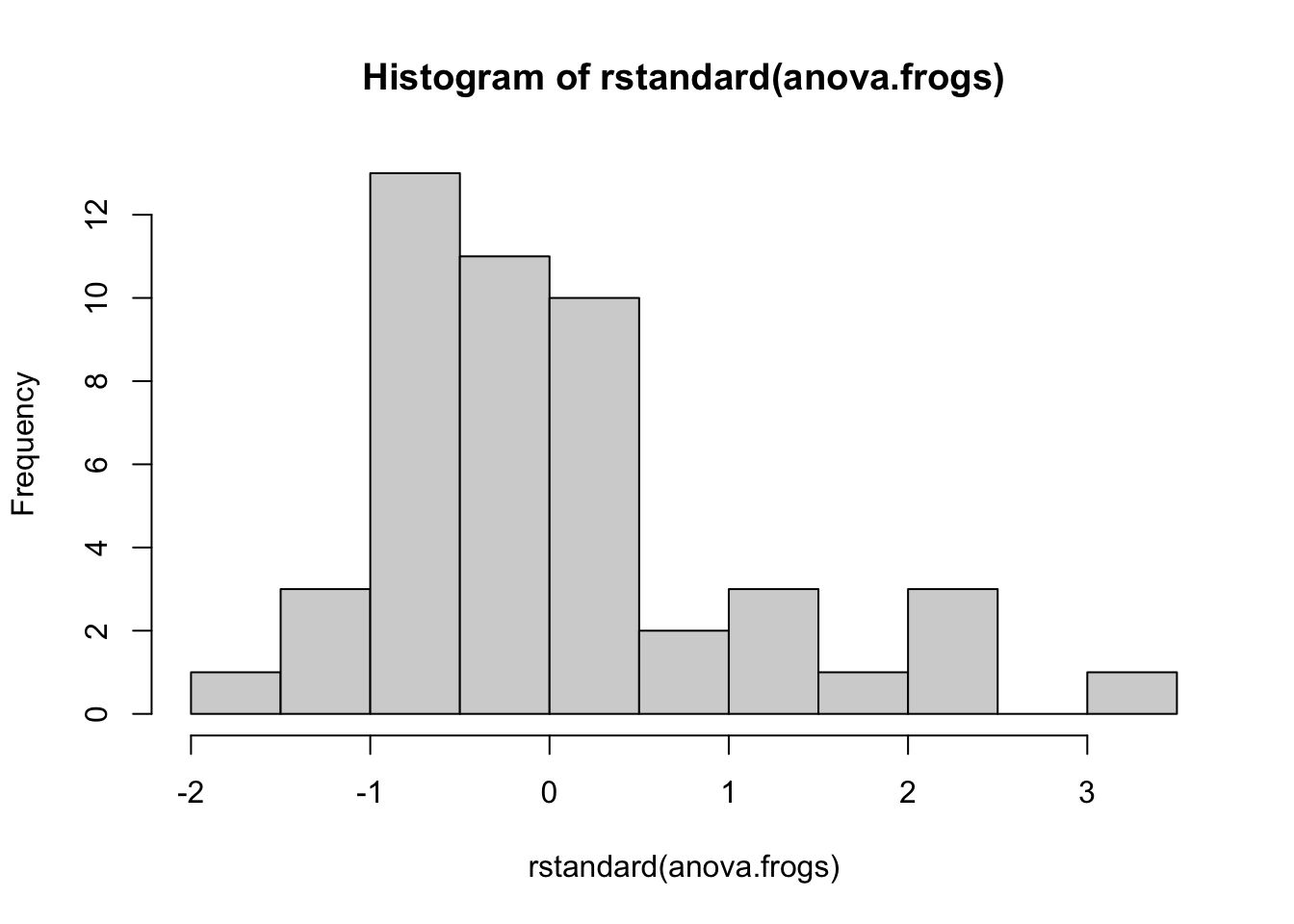
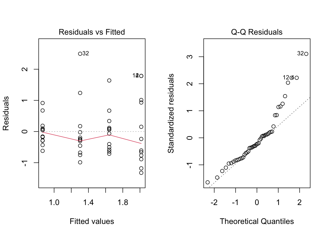
**Histogram of standardised residuals:**
The figure below presents the histogram of the standardised residuals. The majority of the observations show a skew in the distribution.
```{r}
hist(rstandard(anova.frogs))
```
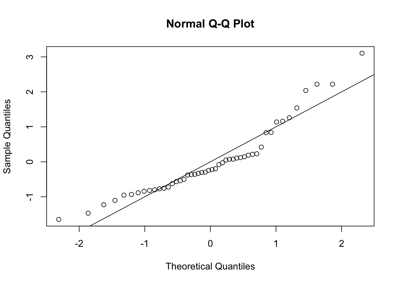
**Q-Q plot:**
The QQ plot below shows that the observed quantiles deviate from the theoretical quantiles (assuming normality). The observations do not follow the line. We can assume the data is not normally distributed.
```{r}
qqnorm(rstandard(anova.frogs))
abline(0, 1)
```
An alternative method for testing normality is to use the Shapiro-Wilk test. This test has the null hypothesis that the data is normally distributed. A p-value < 0.05 indicates we reject the null hypothesis and therefore the data is not normally distributed.
```{r}
shapiro.test(rstandard(anova.frogs))
```
### Part C --- Testing equal variance (homoscedasticity)
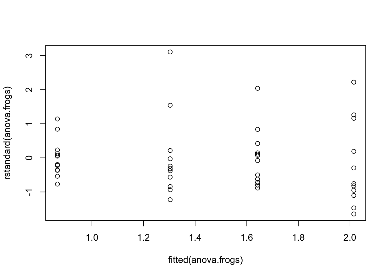
The plot below shows the standardised residuals plotted against the fitted values (the group means in this case). To test the assumption of constant variance we want to have the same spread of observations for increases in the fitted values. We do not want to see *fanning* where the spread of residuals increases or decreases while the fitted values increase. In this case it is hard to see any fanning in this plot - mostly at the beginning, so your conclusion may be that the assumption of equal variance is fine.
```{r}
plot(fitted(anova.frogs), rstandard(anova.frogs))
```
Alternatively we can use the Bartlett test to test for homogeneity of variance using the residuals. The null hypothesis is that the variances are equal across groups. A p-value < 0.05 indicates we reject the null hypothesis and therefore the variances are not equal.
```{r}
bartlett.test(rstandard(anova.frogs) ~ frogs$treatment)
```
Note that sometimes the two approaches may lead to different conclusions...but why?
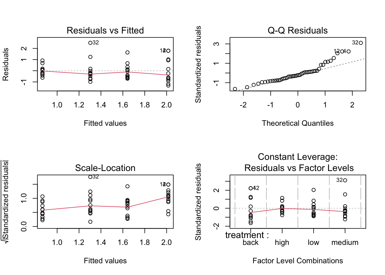
We can also use the built-in `plot()` function to produce the diagnostics plots.
```{r}
par(mfrow = c(2, 2))
plot(anova.frogs)
par(mfrow = c(1, 1))
```
or:
```{r}
par(mfrow = c(1, 2))
plot(anova.frogs, which = 1) # Residuals vs fitted values
plot(anova.frogs, which = 2) # Normal Q-Q plot
par(mfrow = c(1, 1))
```
### Part D --- Transforming the data
If the assumptions of normality and/or homogeneity of variances are not met, we can try transforming the response variable to meet these assumptions. Common transformations include log and square root transformations.
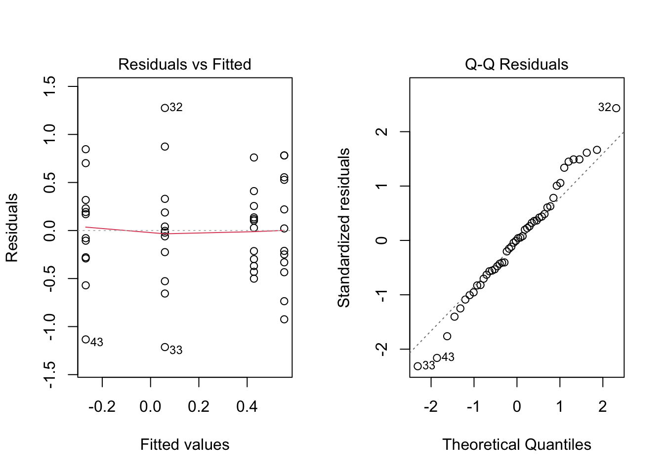
```{r}
anova.log.frogs <- aov(log(shannon_diversity) ~ treatment, data = frogs)

par(mfrow = c(1, 2))
plot(anova.log.frogs, which = 1) # Residuals vs fitted values
plot(anova.log.frogs, which = 2) # Normal Q-Q
par(mfrow = c(1, 1))
```
We can also check the statistical tests for normality and homogeneity of variances on the log-transformed data.
For normality:
```{r}
shapiro.test(rstandard(anova.log.frogs))
```
P>0.05 so we can assume the residuals are normally distributed.
For homogeneity of variances:
```{r}
bartlett.test(rstandard(anova.log.frogs) ~ frogs$treatment)
```
P > 0.05 so we can assume the variances are equal across groups.
We can proceed with the log-transformed data for our ANOVA analysis and post-hoc tests.
::: {.column-margin}
As our models become more complicated, it becomes harder to use the Shapiro-Wilk normality test and Bartlett test of homogeneity of variances. Use graphical methods instead.
:::
ANOVA summary:
```{r}
summary(anova.log.frogs)
```
We can conclude there is a significant effect of treatment on the Shannon diversity of frog communities in streams (p-value = 0.003). This indicates that at least one of the treatment groups has a significantly different mean Shannon diversity compared to the others.
---
### Part E --- Post-hoc tests
::: {.column-margin}
Post-hoc tests are performed after an ANOVA when there are significant differences among group means. The purpose of post-hoc tests is to identify which specific pairs of group means are significantly different from each other. **Do not do a post-hoc test if the ANOVA is not significant!**
:::
We can determine which pairs of treatment means are significantly different. We can do this using Tukey's Honest Significant Difference using the `emmeans` package.
```{r}
library(emmeans)
tukey.frogs <- emmeans(anova.log.frogs, pairwise ~ treatment)
tukey.frogs
```
The output shows the pairwise comparisons between the different Zinc treatments. The `p.value` column indicates whether the differences between the means are statistically significant. A p-value less than 0.05 indicates a significant difference between the treatment means.
From the results, we can see that:
- The comparison between high and low has a p-value of 0.0165, indicating a significant difference in means. The back - high comparison has a p-value of 0.0035, also indicating a significant difference.
- The other comparisons were not significant as their p-values are greater than 0.05.
You can also see the P values have been adjusted for multiple comparisons by the last line in the output.
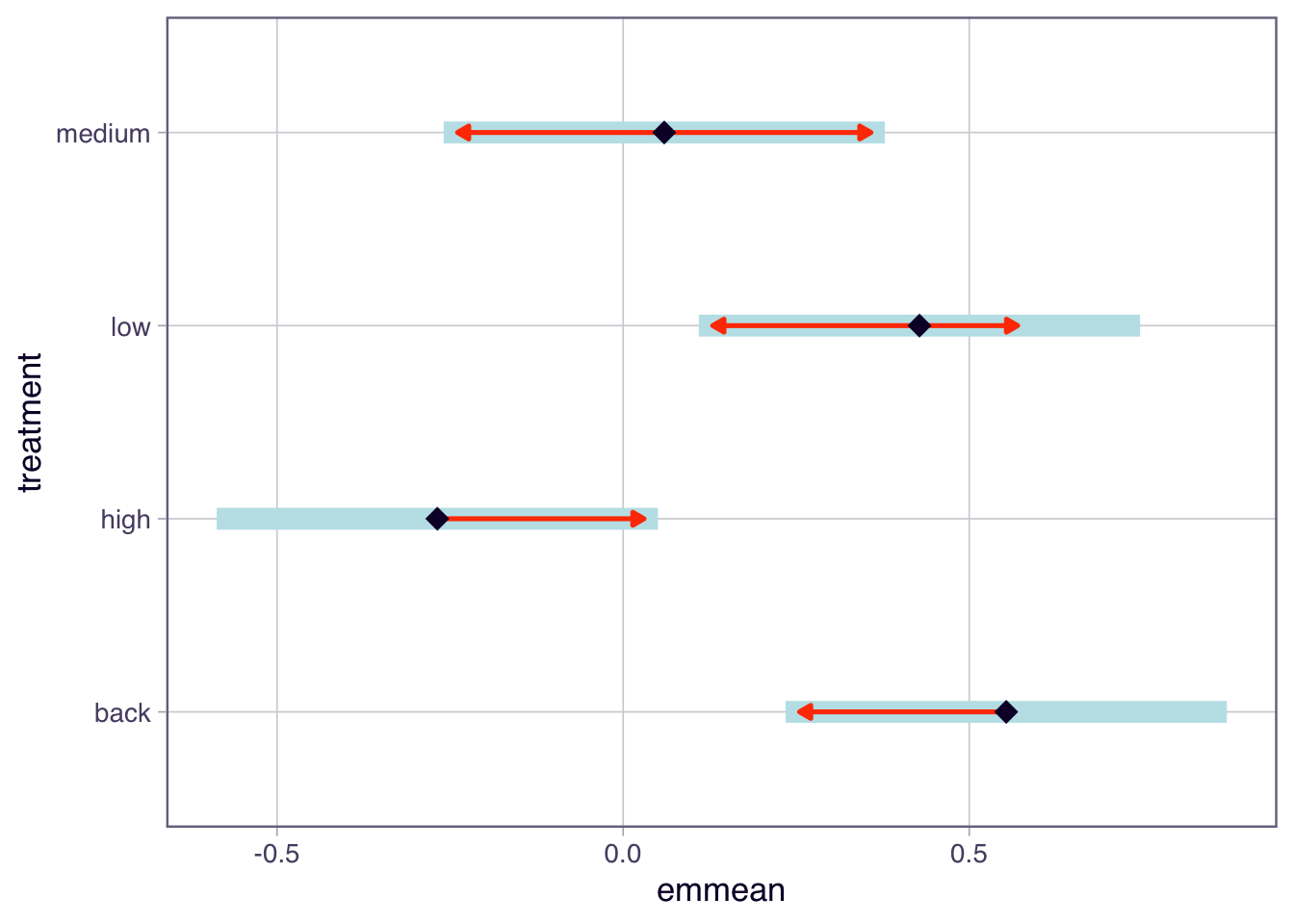
We can also visualise the results using a plot.
```{r}
plot(tukey.frogs, comparisons = TRUE)
```
This plot shows the estimated marginal means (EMM) for each Zinc treatment. In the plot function above, we have specified `comparisons = TRUE`. The blue bars are 95% confidence intervals for the EMMs, and the red arrows are for the comparisons among them (they are adjusted for the multiple comparisons to reduce type 1 errors). If an arrow from one mean overlaps an arrow from another group, the difference is not significant.
Overall, this analysis allows us to identify which Zinc treatments have significantly different effects on frog diversity in streams.
::: {.column-margin}
Statistical tests for multiple comparisons can sometimes be difficult to interpret, especially when there are many groups involved. Hence many propose graphical methods as a more powerful way to determine which groups are different.
:::
::: {.callout-note}
## Checkpoint
We should be able to test ANOVA assumptions using diagnostic plots and formal tests, apply a log transformation when assumptions are violated, and use Tukey's test to identify which groups differ.
:::
# Multiple comparisons and the error-power trade-off
## Exercise 3: Family-wise error rate and power {.unnumbered}
When conducting multiple pairwise comparisons, the family-wise error rate increases. To control the family-wise error rate, post-hoc tests like Tukey's HSD are used, which adjust the significance levels to account for the number of comparisons being made.
::: {.column-margin}
The family-wise error rate is the probability of making at least one Type I error (false positive) among all the comparisons.
:::
Tukey's HSD test is designed to maintain the overall family-wise error rate at a specified level (commonly 0.05) while still providing sufficient power to detect true differences between group means.
However, there is a trade-off between controlling the family-wise error rate and maintaining statistical power. As the number of comparisons increases, the adjustments made by post-hoc tests can lead to a reduction in power, making it more difficult to detect true differences.
Therefore, it is important to carefully consider the number of comparisons being made and choose appropriate post-hoc tests that balance the need for controlling Type I errors with the desire to maintain adequate statistical power.
### Part A --- Tukey-adjusted comparisons
We can look at an example of the trade-off between family-wise error rate and power using simulation.
```{r}
set.seed(123)
n_groups <- 5
n_per_group <- 10
n_simulations <- 1000
alpha <- 0.05
family_wise_errors <- 0

for (i in 1:n_simulations) {
  data <- data.frame(
    value = rnorm(n_groups * n_per_group, mean = 0, sd = 1),
    group = as.factor(rep(1:n_groups, each = n_per_group))
  )

  anova_model <- aov(value ~ group, data = data)
  tukey_result <- TukeyHSD(anova_model)

  if (any(tukey_result$group[, "p adj"] < alpha)) {
    family_wise_errors <- family_wise_errors + 1
  }
}
family_wise_error_rate <- family_wise_errors / n_simulations
family_wise_error_rate
```
In this simulation, we create 5 groups with 10 observations each, and we run 1000 simulations. We fit a one-way ANOVA model to the data and perform Tukey's HSD test for pairwise comparisons. We count how many times at *least one comparison is significant (p-value < 0.05)* across all simulations to estimate the family-wise error rate (~0.04 or 4% error rate).
The resulting family-wise error rate should be close to the nominal level of 0.05, demonstrating that Tukey's HSD test effectively controls the family-wise error rate while maintaining reasonable power to detect true differences between group means.
### Part B --- Unadjusted t-tests
If we do not use a post-hoc test and just do multiple t-tests we can see how the family-wise error rate increases. For example, we will not adjust the p-values for multiple comparisons:
```{r}
family_wise_errors_no_adjust <- 0
for (i in 1:n_simulations) {
  data <- data.frame(
    value = rnorm(n_groups * n_per_group, mean = 0, sd = 1),
    group = as.factor(rep(1:n_groups, each = n_per_group))
  )

  p_values <- c()
  for (j in 1:(n_groups - 1)) {
    for (k in (j + 1):n_groups) {
      t_test_result <- t.test(value ~ group, data = subset(data, group %in% c(j, k)))
      p_values <- c(p_values, t_test_result$p.value)
    }
  }

  if (any(p_values < alpha)) {
    family_wise_errors_no_adjust <- family_wise_errors_no_adjust + 1
  }
}
family_wise_error_rate_no_adjust <- family_wise_errors_no_adjust / n_simulations
family_wise_error_rate_no_adjust
```
In this simulation, we perform multiple t-tests without adjusting the p-values for multiple comparisons. We count how many times at *least one comparison is significant (p-value < 0.05)* across all simulations to estimate the family-wise error rate.
The resulting family-wise error rate should be significantly higher than the nominal level of 0.05 (i.e. ~0.286 or 29% error rate!), demonstrating that not adjusting for multiple comparisons leads to an increased risk of Type I errors.
This example highlights the importance of using post-hoc tests like Tukey's HSD to control the family-wise error rate when conducting multiple pairwise comparisons in ANOVA.
### Part C --- Power trade-off
::: {.column-margin}
Statistical power is the probability of correctly rejecting the null hypothesis when it is false (i.e., detecting a true effect).
:::
When conducting multiple comparisons, there is a trade-off between controlling the family-wise error rate and maintaining statistical power. As the number of comparisons increases, the adjustments made by post-hoc tests can lead to a reduction in power, making it more difficult to detect true differences.
To illustrate this trade-off, we can simulate data with a known effect size and compare the power of Tukey's HSD test to that of unadjusted t-tests.
```{r}
set.seed(123)
n_groups <- 5
n_per_group <- 10
n_simulations <- 1000
alpha <- 0.05
true_effect_size <- 1
power_tukey <- 0
power_t_test <- 0
for (i in 1:n_simulations) {
  data <- data.frame(
    value = c(rnorm(n_per_group, mean = 0, sd = 1),
              rnorm(n_per_group, mean = true_effect_size, sd = 1),
              rnorm(n_per_group, mean = 0, sd = 1),
              rnorm(n_per_group, mean = 0, sd = 1),
              rnorm(n_per_group, mean = 0, sd = 1)),
    group = as.factor(rep(1:n_groups, each = n_per_group))
  )

  anova_model <- aov(value ~ group, data = data)
  tukey_result <- TukeyHSD(anova_model)

  if (tukey_result$group["2-1", "p adj"] < alpha) {
    power_tukey <- power_tukey + 1
  }

  t_test_result <- t.test(value ~ group, data = subset(data, group %in% c(1, 2)))
  if (t_test_result$p.value < alpha) {
    power_t_test <- power_t_test + 1
  }
}
power_tukey_rate <- power_tukey / n_simulations
power_t_test_rate <- power_t_test / n_simulations
```
```{r}
# print results:
cat("Adjusted for family-rate errors using Tukey's test. Proportion correctly detected:", power_tukey_rate, "\n")
cat("Unadjusted t-tests. Proportion correctly detected:", power_t_test_rate, "\n")
```
In this simulation, we create 5 groups with 10 observations each, where one group has a true effect size of 1. We run 1000 simulations and fit a one-way ANOVA model to the data. We then perform Tukey's HSD test and unadjusted t-tests to compare the power of each method in detecting the true effect.
The resulting power rates indicate the proportion of simulations in which each method correctly detected the true effect. We expect the power of the unadjusted t-tests to be *higher (~57%)* than that of Tukey's HSD test *(\~30%)*, demonstrating the trade-off between controlling the family-wise error rate and maintaining statistical power.
### Part D --- Explore the trade-off
The simulations above used 5 groups. Use the widget below to see how the trade-off changes as the number of groups increases.
```{=html}
<style>
#part-d-explore-the-trade-off .cell-output-display {
border: none;
padding: 0;
margin: 0;
}
</style>
```
```{ojs}
//| echo: false
import { fwePowerWidget } from "../assets/js/fwe-power-widget.js"
fwePowerWidget()
```
::: {.callout-note}
## Checkpoint
We should be able to explain the trade-off between controlling the family-wise error rate and maintaining statistical power, and why Tukey's test is preferred over unadjusted t-tests for multiple comparisons.
:::
## Wrap-up {.unnumbered}
We covered the use of residuals for checking ANOVA assumptions, applied diagnostic tools to a real dataset, and explored how post-hoc tests balance error control with statistical power. In the lab, we will apply these techniques to new datasets and practise interpreting back-transformed results.