Welcome
In this tutorial we will explore experimental design principles by testing randomisation with a class activity, then analysing simulated CRD and RCBD experiments in R.
You will learn how to:
- Assess the validity of an experiment in terms of randomisation, experimental units, and replication.
- Analyse a completely randomised design (CRD) using ANOVA.
- Analyse a randomised complete block design (RCBD) and calculate the percentage of variation explained by treatments and blocks.
1 Randomisation
Randomisation is a key principle of experimental design. It helps to ensure that the treatment groups are comparable and that the results of the experiment are not biased by confounding factors.
- It helps to eliminate bias in the allocation of treatments to experimental units.
- It helps to ensure that the treatment groups are comparable.
- It helps to ensure that the results of the experiment are not confounded by other factors.
- It is a key assumption of all statistical models.
Exercise 1: Testing randomisation
Let us work together as a class to test the effect of randomisation on an experiment. We will simulate an experiment with and without randomisation and compare the results.
Assign each student a number from 1 to the total number of students in the class. Each student will be asked to answer the question:
“Do you know the student next to you? Yes or No”
Part A — Non-random sample
“Do you know the student next to you? Yes or No”
Put your hand up if you answer “Yes”, and keep it down if you answer “No”. The students with their hands up are counted as “Yes” and the students with their hands down are counted as “No”. This is our non-random sample.
Class answers — Replace these with your class numbers:
Class size (number of students present):
Part B — Percentages from the non-random sample
Part C — Random sample
We simulate student IDs and assign a random number to each ID.
Random sample size (how many students you will sample at random):
Randomly select students:
 [1] 16 46 40  8  6 60 22 36 45 57 33 51 55 11 27 43 41 25 49 54 47 24 29 39 59
[26] 17 13  1 50  4
“Do you know the student next to you? Yes or No”
Enter counts for the random sample:
After you randomly select those students and ask the question, enter the counts here.
Percentages for the random sample:
Random sample % Yes: 46.7 %Random sample % No : 53.3 %Estimate the bias:
Bias here is the difference between the non-random sample proportion and the random sample proportion.
Estimated bias in % Yes (non-random - random): 16.7 %Estimated bias in % No (non-random - random): -16.7 %Visualisation:
Bar plot of % Yes/No for non-random vs random samples using ggplot2.
percent_df <- data.frame(
  sample_type = rep(c("Non-random", "Random"), each = 2),
  response    = rep(c("Yes", "No"), times = 2),
  percent     = c(prop_yes_nonrandom, prop_no_nonrandom, prop_yes_random, prop_no_random)
)

library(ggplot2)

ggplot(percent_df, aes(x = response, y = percent, fill = sample_type)) +
  geom_col(position = "dodge") +
  labs(x = "Response", y = "Percent", fill = "Sample type")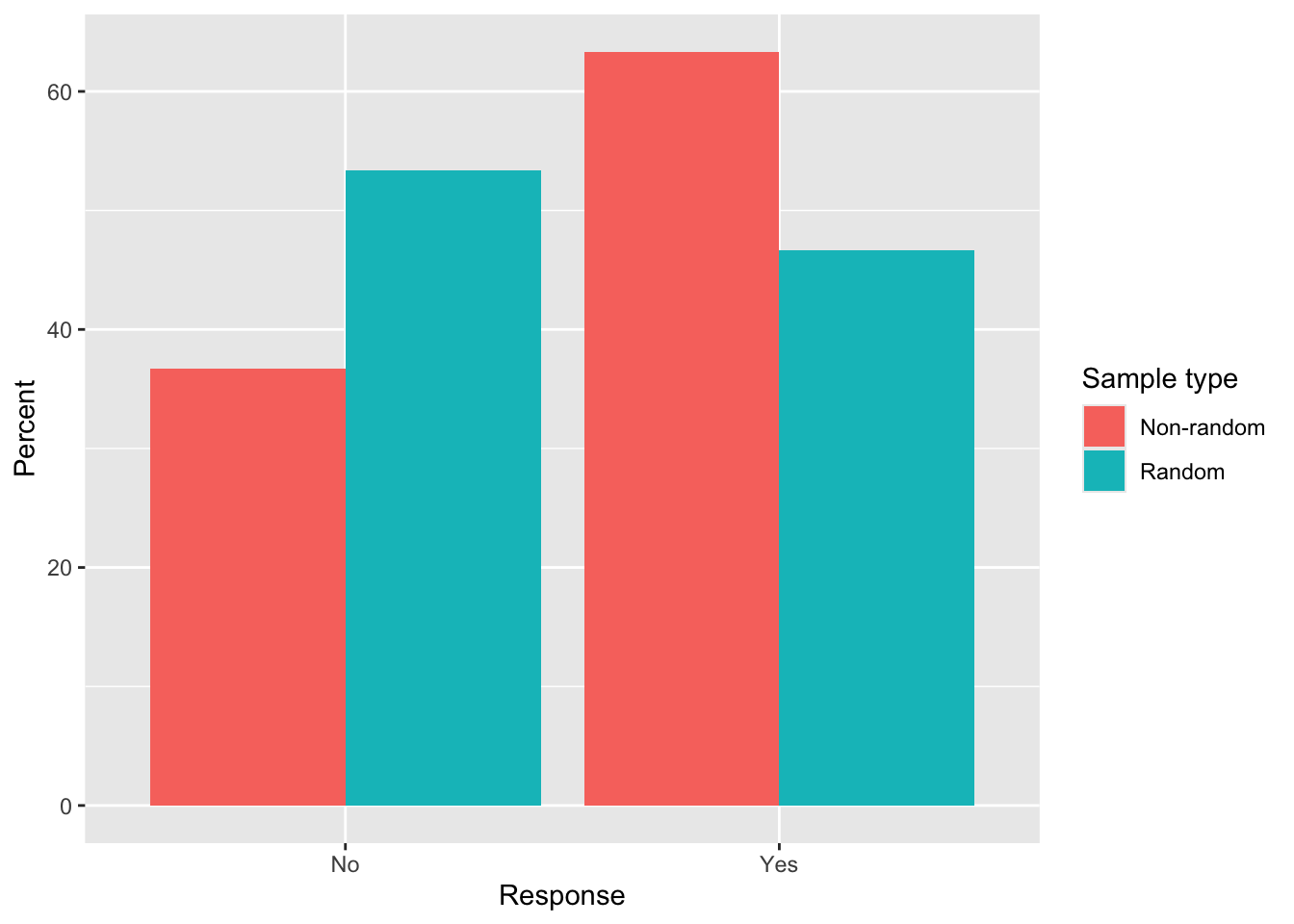
Non-random sampling (asking about the person next to you) is typically biased because seating patterns cluster friends or cohorts.
- Random sampling gives each student an equal chance, reducing systematic bias.
- Comparing the two percentages provides a simple measure of bias in this context.
You should now be able to explain why random sampling reduces bias compared to convenience sampling, and how to estimate the magnitude of that bias.
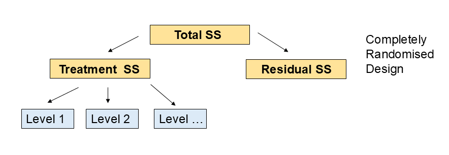
2 Control of variation: CRD
In a Completely Randomised Design (CRD), experimental units are randomly assigned to treatments. This design is appropriate when the experimental units are homogeneous and there are no known sources of variation that need to be controlled.
- Random assignment of treatments to experimental units.
- Appropriate for homogeneous experimental units.
- Simple to implement and analyse.
Simple experiments can be easier to interpret, but may not control for variation as well as more complex designs.
Exercise 2: CRD
Consider an experiment to test the effect of different fertilizers on plant growth using a CRD. The experiment uses 12 pots, with 4 pots assigned to each of 3 fertilizer treatments (A, B, and C). Each pot contains 5 plants, and the height of each plant is measured after 4 weeks.
The statistical model for this CRD can be expressed as: Y_{ij} = \mu + \alpha_i + \epsilon_{ij} Where:
- Y_{ij} is the observed height of the j-th plant in the i-th fertilizer treatment.
- \mu is the overall mean height across all fertilizer treatments.
- \alpha_i is the effect of the i-th fertilizer treatment (i = A, B, C).
- \epsilon_{ij} is the random error associated with the j-th plant in the i-th treatment, assumed to be independently and identically distributed with mean 0 and variance \sigma^2.
OR:
Plant\ height = overall\ mean + fertilizer\ treatment + random\ error.
Show the code
   pot_id treatment
1       1         A
2       2         C
3       3         C
4       4         A
5       5         B
6       6         C
7       7         B
8       8         A
9       9         C
10     10         B
11     11         A
12 12 B- The treatments are randomly assigned to the pots.
- The height of each plant is measured after 4 weeks.
Show the code
   pot_id plant_id    height treatment
1       1        1  7.312957         A
2       1        2 11.243551         A
3       1        3 11.601749         A
4       1        4  7.222215         A
5       1        5  8.571286         A
6       2        6  9.351878         C
7       2        7 11.381286         C
8       2        8 10.501096         C
9       2        9 12.014705         C
10      2       10 11.146469         C
11      3       11  8.168379         C
12      3       12 12.622195         C
13      3       13 11.977453         C
14      3       14 13.307857         C
15      3       15  7.118390         C
16      4       16 13.894713         A
17      4       17 13.473872         A
18      4       18 10.774967         A
19      4       19 14.560068         A
20      4       20 13.075767         A
21      5       21 14.050792         B
22      5       22 11.565382         B
23      5       23 12.146339         B
24      5       24 15.416472         B
25      5       25 14.928328         B
26      6       26 17.268569         C
27      6       27 14.074290         C
28      6       28 14.343232         C
29      6       29 17.969079         C
30      6       30 12.821244         C
31      7       31 13.942412         B
32      7       32 13.812414         B
33      7       33 11.002169         B
34      7       34 15.592306         B
35      7       35 15.341251         B
36      8       36 18.631305         A
37      8       37 13.678794         A
38      8       38 14.719496         A
39      8       39 14.152042         A
40      8       40 14.922528         A
41      9       41 19.942116         C
42      9       42 20.786075         C
43      9       43 19.500772         C
44      9       44 20.166900         C
45      9       45 24.157749         C
46     10       46 20.241704         B
47     10       47 20.236299         B
48     10       48 21.540108         B
49     10       49 17.649195         B
50     10       50 20.818077         B
51     11       51 18.670098         A
52     11       52 19.486950         A
53     11       53 21.357564         A
54     11       54 21.793689         A
55     11       55 21.236713         A
56     12       56 21.462907         B
57     12       57 19.173651         B
58     12       58 23.115626         B
59     12       59 21.083398         B
60 12 60 21.154301 B- The data can be analysed using ANOVA to test for differences in plant height between the fertilizer treatments.
Is there a significant difference in plant height between the fertilizer treatments?
            Df Sum Sq Mean Sq F value Pr(>F)
treatment    2  100.1   50.04   2.641   0.08 .
Residuals   57 1080.2   18.95
---
Signif. codes: 0 '***' 0.001 '**' 0.01 '*' 0.05 '.' 0.1 ' ' 1- The ANOVA results will indicate whether there are significant differences in plant height between the fertilizer treatments.
You should now be able to write out a CRD statistical model, fit it using aov(), and interpret the ANOVA output to determine whether there are significant treatment effects.
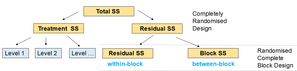
3 Control of variation: RCBD
In a Randomised Complete Block Design (RCBD), experimental units are grouped into blocks based on known sources of variation, and treatments are randomly assigned within each block. This design is appropriate when there are known sources of variation that need to be controlled.
- Grouping of experimental units into blocks.
- Random assignment of treatments within blocks.
- Appropriate for heterogeneous experimental units.
Exercise 3: RCBD
Consider an experiment to test the effect of different fertilizers on plant growth using an RCBD. The experiment uses 12 pots, with 4 pots assigned to each of 3 fertilizer treatments (A, B, and C). The pots are grouped into 4 blocks based on their location in the greenhouse (North, South, East, West). Each pot contains 5 plants, and the height of each plant is measured after 4 weeks.
The statistical model for this RCBD can be expressed as: Y_{ijk} = \mu + \beta_j + \alpha_i + \epsilon _{ijk} Where:
- Y_{ijk} is the observed height of the k-th plant in the i-th fertilizer treatment and j-th block.
- \mu is the overall mean height across all fertilizer treatments and blocks.
- \beta_j is the effect of the j-th block (j = North, South, East, West).
- \alpha_i is the effect of the i-th fertilizer treatment (i = A, B, C).
- \epsilon_{ijk} is the random error associated with the k-th plant in the i-th treatment and j-th block, assumed to be independently and identically distributed with mean 0 and variance \sigma^2.
OR:
Plant\ height = overall\ mean + block + fertilizer\ treatment + random\ error.
Show the code
   pot_id block treatment
1       1 North         C
2       2 North         C
3       3 North         A
4       4 South         B
5       5 South         C
6       6 South         B
7       7  East         B
8       8  East         A
9       9  East         C
10     10  West         B
11     11  West         A
12 12 West A- The treatments are randomly assigned to the pots within each block.
- The height of each plant is measured after 4 weeks.
Show the code
   pot_id plant_id    height block treatment
1       1        1  9.312957 North         C
2       1        2 13.243551 North         C
3       1        3 13.601749 North         C
4       1        4  9.222215 North         C
5       1        5 10.571286 North         C
6       2        6 11.351878 North         C
7       2        7 13.381286 North         C
8       2        8 12.501096 North         C
9       2        9 14.014705 North         C
10      2       10 13.146469 North         C
11      3       11 10.168379 North         A
12      3       12 14.622195 North         A
13      3       13 13.977453 North         A
14      3       14 15.307857 North         A
15      3       15  9.118390 North         A
16      4       16 11.894713 South         B
17      4       17 11.473872 South         B
18      4       18  8.774967 South         B
19      4       19 12.560068 South         B
20      4       20 11.075767 South         B
21      5       21 12.050792 South         C
22      5       22  9.565382 South         C
23      5       23 10.146339 South         C
24      5       24 13.416472 South         C
25      5       25 12.928328 South         C
26      6       26 15.268569 South         B
27      6       27 12.074290 South         B
28      6       28 12.343232 South         B
29      6       29 15.969079 South         B
30      6       30 10.821244 South         B
31      7       31 14.942412  East         B
32      7       32 14.812414  East         B
33      7       33 12.002169  East         B
34      7       34 16.592306  East         B
35      7       35 16.341251  East         B
36      8       36 19.631305  East         A
37      8       37 14.678794  East         A
38      8       38 15.719496  East         A
39      8       39 15.152042  East         A
40      8       40 15.922528  East         A
41      9       41 20.942116  East         C
42      9       42 21.786075  East         C
43      9       43 20.500772  East         C
44      9       44 21.166900  East         C
45      9       45 25.157749  East         C
46     10       46 19.241704  West         B
47     10       47 19.236299  West         B
48     10       48 20.540108  West         B
49     10       49 16.649195  West         B
50     10       50 19.818077  West         B
51     11       51 17.670098  West         A
52     11       52 18.486950  West         A
53     11       53 20.357564  West         A
54     11       54 20.793689  West         A
55     11       55 20.236713  West         A
56     12       56 20.462907  West         A
57     12       57 18.173651  West         A
58     12       58 22.115626  West         A
59     12       59 20.083398  West         A
60     12       60 20.154301  West         A
The data can be analysed using ANOVA to test for differences in plant height between the fertilizer treatments while accounting for block effects.
            Df Sum Sq Mean Sq F value   Pr(>F)
block        3  664.5  221.50  41.589 4.59e-14 ***
treatment    2   33.5   16.77   3.148   0.0509 .
Residuals   54  287.6    5.33
---
Signif. codes:  0 '***' 0.001 '**' 0.01 '*' 0.05 '.' 0.1 ' ' 1
The ANOVA results will indicate whether there are significant differences in plant height between the fertilizer treatments while controlling for block effects.
The percentage of variation explained by treatments and blocking terms can be calculated from the ANOVA table.
- Sum of Squares (SS) for each source of variation can be found in the ANOVA table.
- Percentage of variation explained by a source = (SS for that source / Total SS) × 100
For example, to calculate the percentage of variation explained by treatments and blocks:
- SS_total = Sum of Squares Total
- SS_treatment = Sum of Squares for Treatment
- SS_block = Sum of Squares for Block
Percentage of variation explained by treatments = (SS_treatment / SS_total) × 100
Percentage of variation explained by blocks = (SS_block / SS_total) × 100
We are using R to subset the ANOVA results to calculate these percentages, but you can do this by hand from the ANOVA table using a calculator. Try this and compare your answers to the results from the code below.
You will need to know how to read the ANOVA table and calculate the percentage variation explained by hand for your assessments.
anova_table <- summary(anova_result)[[1]]
ss_total <- sum(anova_table$`Sum Sq`)
ss_treatment <- anova_table$`Sum Sq`[2]
ss_block <- anova_table$`Sum Sq`[1]
percent_treatment <- (ss_treatment / ss_total) * 100
percent_block <- (ss_block / ss_total) * 100
cat("Percentage of variation explained by treatments:", round(percent_treatment, 1), "%\n")
Percentage of variation explained by treatments: 3.4 %Percentage of variation explained by blocks: 67.4 %This information helps to understand the contribution of treatments and blocks to the overall variation in plant height.
You should now be able to write out an RCBD statistical model, fit it using aov() with a blocking term, interpret the output, and calculate the percentage of variation explained by treatments and blocks from the ANOVA table.
Wrap-up
In this tutorial, we covered key concepts in experimental design, including randomisation, experimental units vs sampling units, replication, and control of variation through CRD and RCBD. We also demonstrated how to analyse data from these designs using ANOVA in R.
Example exam questions
Define the terms “experimental unit” and “sampling unit”. Provide an example of each from a hypothetical agricultural experiment.
Explain the importance of randomisation in experimental design. How does randomisation help to reduce bias in an experiment?
Describe the key features of a Completely Randomised Design (CRD). When is it appropriate to use a CRD?
Describe the key features of a Randomised Complete Block Design (RCBD). When is it appropriate to use an RCBD?
Given an ANOVA table from an RCBD experiment, calculate the percentage of variation explained by treatments and blocks.