---
title: "Tutorial 06"
# reviewed-by:
format:
sandstone-html:
code-tools: true
---
```{r setup, include=FALSE}
knitr::opts_chunk$set(echo = TRUE)
```
## Welcome {.unnumbered}
In this week's lectures we covered factorial designs, main effects and interactions. We applied these concepts by using analysis of variance (ANOVA) as a method to analyse data from these experimental designs.
You will learn how to:
1. Distinguish between treatment designs and experimental designs.
2. Identify main effects and interactions in factorial treatment structures, including graphical interpretations.
3. Perform ANOVA with factorial treatment designs, with and without blocking.
# Treatment designs and experimental designs
An experimental design is a structured approach to conducting experiments that allows researchers to systematically investigate the effects of one or more factors on a response variable. Treatment designs refer to the specific arrangements of treatments (or interventions) applied to experimental units within an experimental design. There are several types of treatment designs, including (but not limited to):
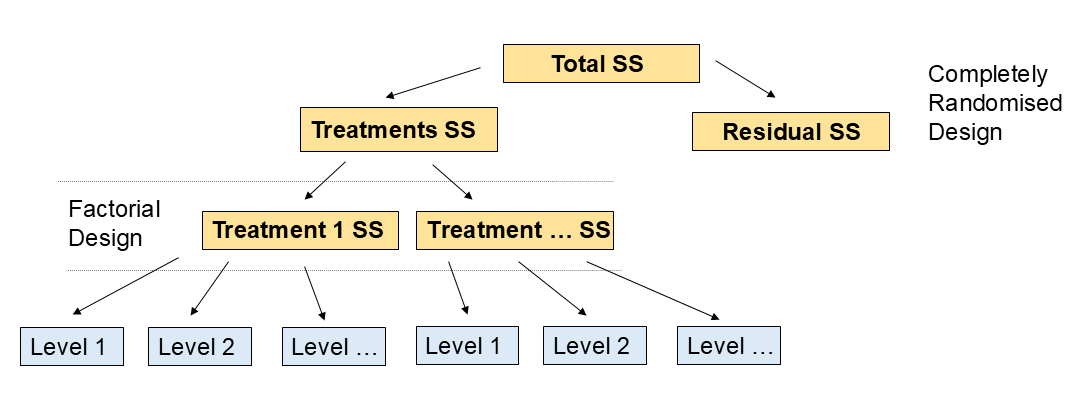
- **Completely Randomised Design (CRD)**: Experimental units are randomly assigned to different treatment groups without any restrictions. This design is suitable when experimental units are homogeneous.
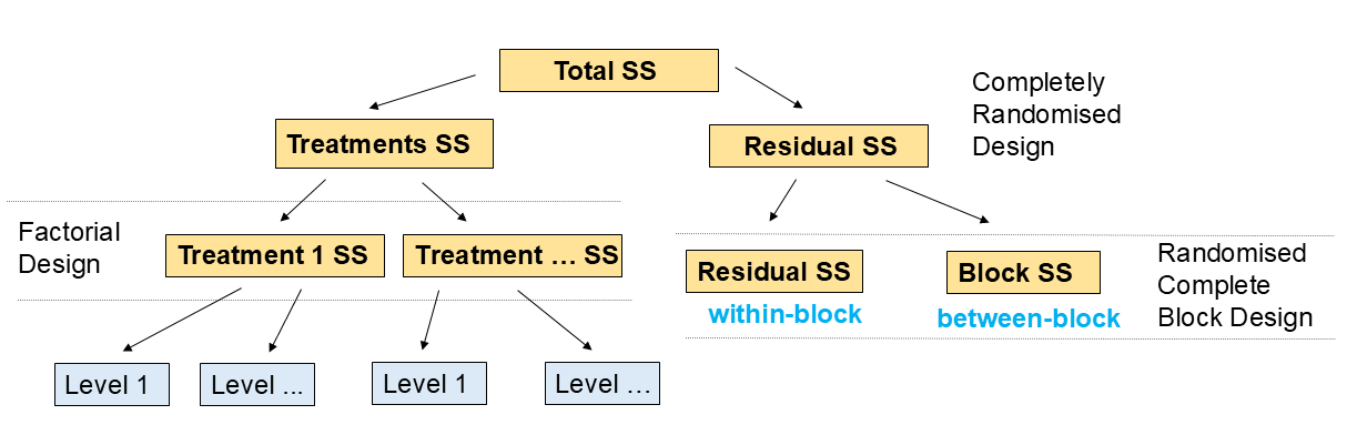
- **Randomised Block Design (RBD)**: Experimental units are grouped into blocks based on certain characteristics, and treatments are randomly assigned within each block. This design helps control for variability among experimental units.
- **Factorial Design**: Multiple factors are investigated simultaneously, with all possible combinations of factor levels included in the experiment. This design allows for the study of main effects and interactions between factors.
# Factorial treatment structure
Factorial treatment structures involve experiments where there are two or more treatment factors, each with two or more levels. In these designs, all possible combinations of the levels of each factor are included in the experiment. For example, in a 2-way factorial design with factors A and B, where factor A has 2 levels (A1 and A2) and factor B has 3 levels (B1, B2, and B3), the treatment combinations would be A1B1, A1B2, A1B3, A2B1, A2B2, and A2B3.
## Main effects and interactions
In a factorial design, the **main effects** refer to the individual effects of each treatment/factor on the response variable, while **interactions** refer to the combined effects of two or more treatments/factors on the response variable. An interaction occurs when the effect of one treatment/factor depends on the level of another treatment/factor.
Let us plot some examples of interaction plots:
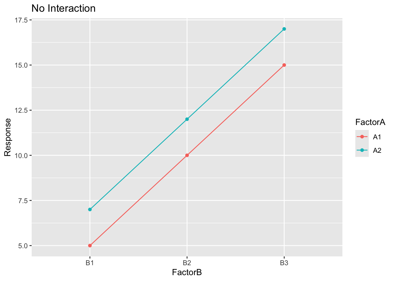
- No interaction
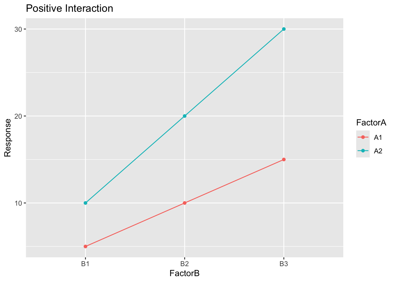
- Positive interaction
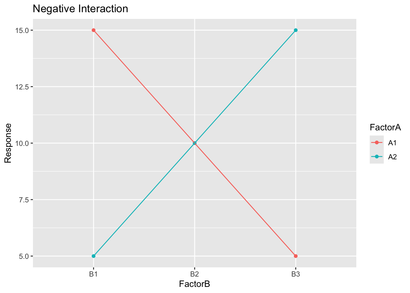
- Negative interaction
```{r}
#| code-fold: true
library(ggplot2)

# No interaction
no_interaction <- data.frame(
  FactorA = rep(c("A1", "A2"), each = 3),
  FactorB = rep(c("B1", "B2", "B3"), times = 2),
  Response = c(5, 10, 15, 7, 12, 17)
)

ggplot(no_interaction, aes(x = FactorB, y = Response, color = FactorA, group = FactorA)) +
  geom_point() +
  geom_line() +
  labs(title = "No Interaction")
# Positive interaction
positive_interaction <- data.frame(
  FactorA = rep(c("A1", "A2"), each = 3),
  FactorB = rep(c("B1", "B2", "B3"), times = 2),
  Response = c(5, 10, 15, 10, 20, 30)
)

ggplot(positive_interaction, aes(x = FactorB, y = Response, color = FactorA, group = FactorA)) +
  geom_point() +
  geom_line() +
  labs(title = "Positive Interaction")
# Negative interaction
negative_interaction <- data.frame(
  FactorA = rep(c("A1", "A2"), each = 3),
  FactorB = rep(c("B1", "B2", "B3"), times = 2),
  Response = c(15, 10, 5, 5, 10, 15)
)

ggplot(negative_interaction, aes(x = FactorB, y = Response, color = FactorA, group = FactorA)) +
  geom_point() +
  geom_line() +
  labs(title = "Negative Interaction")
```
The plots above illustrate different types of interactions between two factors:
- In the **"No Interaction"** plot, the lines are parallel, indicating that the effect of one factor does not depend on the level of the other factor.
- In the **"Positive Interaction"** plot, the lines diverge, indicating that the effect of one factor increases with the level of the other factor.
- In the **"Negative Interaction"** plot, the lines converge, indicating that the effect of one factor decreases with the level of the other factor.
::: callout-tip
## Interpreting interaction plots
- Parallel lines indicate **no interaction** between factors.
- Non-parallel lines indicate an **interaction** between factors.
:::
## Exercise 1: Identifying main effects and interactions {.unnumbered}
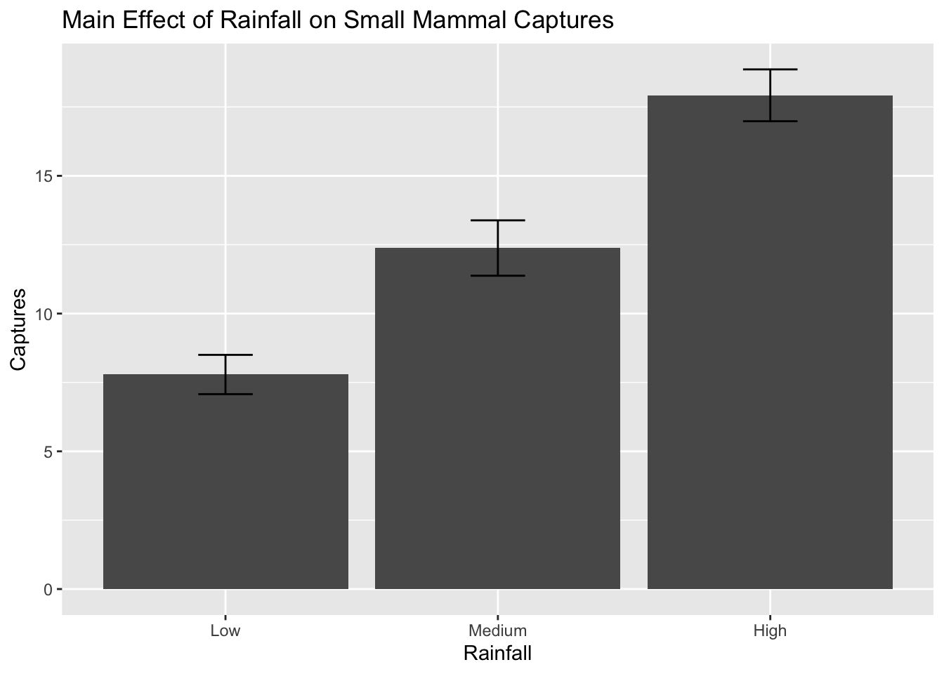
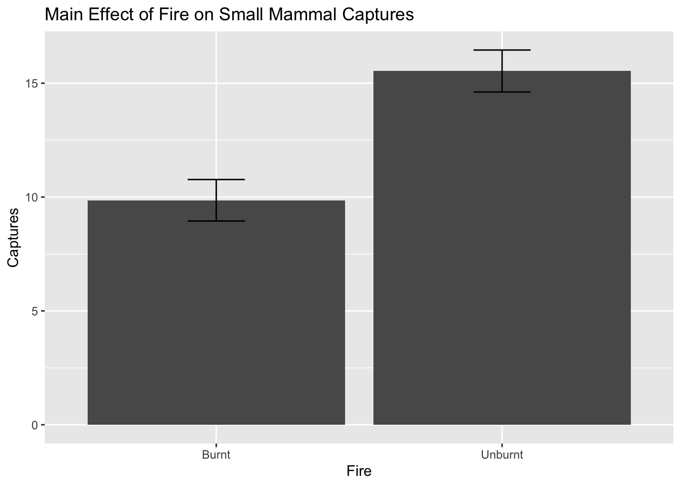
In this ecological experiment, we investigated the influence of two factors: Fire and Rainfall on small mammal captures (using a 2-way factorial design).

Our main effects are:
- Effect of Fire (Levels: Burnt, Unburnt)
- Effect of Rainfall (Levels: Low, Medium, High)
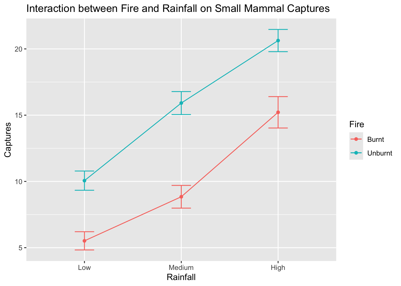
Our interaction is:
- Interaction between Fire and Rainfall
The statistical model for this experiment can be written as:
$$
Y_{ijk} = \mu + \alpha_i + \beta_j + (\alpha\beta)_{ij} + \epsilon_{ijk}
$$
Where:
- $Y_{ijk}$ is the response variable (small mammal captures) for the $k$th observation in the $i$th level of Fire and $j$th level of Rainfall\
- $\mu$ is the overall mean small mammal captures\
- $\alpha_i$ is the effect of the $i$th level of Fire (Burnt vs Unburnt)\
- $\beta_j$ is the effect of the $j$th level of Rainfall (Low, Medium, High)\
- $(\alpha\beta)_{ij}$ is the interaction effect between Fire and Rainfall\
- $\epsilon_{ijk}$ is the random error term for the $k$th observation in the $i$th level of Fire and $j$th level of Rainfall and is assumed to be normally distributed with mean 0 and constant variance $\sigma^2$.\
OR in words:
$$Small\ mammal\ captures = overall\ mean + Fire + Rainfall + Fire \times Rainfall + random\ error$$
Let us simulate some data and plot the main effects and interactions:
```{r}
#| code-fold: true
set.seed(123)
fire <- rep(c("Burnt", "Unburnt"), each = 30)
rainfall <- rep(c("Low", "Medium", "High"), times = 20)
captures <- rnorm(60, mean = ifelse(fire == "Burnt",
                                    ifelse(rainfall == "Low", 5,
                                           ifelse(rainfall == "Medium", 10, 15)),
                                    ifelse(rainfall == "Low", 10,
                                           ifelse(rainfall == "Medium", 15, 20))), sd = 3)

data <- data.frame(Fire = fire, Rainfall = rainfall, Captures = captures)

# Add level order for plotting
data$Rainfall <- factor(data$Rainfall, levels = c("Low", "Medium", "High"))

library(ggplot2)

# Plot main effect: Rainfall
ggplot(data, aes(x = Rainfall, y = Captures)) +
  stat_summary(fun = mean, geom = "bar", aes(group = 1)) +
  stat_summary(fun.data = mean_se, geom = "errorbar", width = 0.2) +
  labs(title = "Main Effect of Rainfall on Small Mammal Captures")
# Plot main effect: Fire
ggplot(data, aes(x = Fire, y = Captures)) +
  stat_summary(fun = mean, geom = "bar", aes(group = 1)) +
  stat_summary(fun.data = mean_se, geom = "errorbar", width = 0.2) +
  labs(title = "Main Effect of Fire on Small Mammal Captures")
# Plot interaction
ggplot(data, aes(x = Rainfall, y = Captures, color = Fire, group = Fire)) +
  stat_summary(fun = mean, geom = "point") +
  stat_summary(fun = mean, geom = "line") +
  stat_summary(fun.data = mean_se, geom = "errorbar", width = 0.2) +
  labs(title = "Interaction between Fire and Rainfall on Small Mammal Captures")
```
::: callout-tip
## Key concepts
- Main effects represent the individual impact of each factor on the response variable.
- Interactions occur when the effect of one factor depends on the level of another factor.
- **If an interaction is significant, do not interpret the main effects on their own.**
- Read a factorial ANOVA table from the bottom up: interaction terms first, then main effects.
You must understand these concepts to correctly interpret the results of factorial experiments.
:::
::: {.callout-note}
## Checkpoint
You should now be able to identify main effects and interactions from interaction plots, and write out a statistical model for a two-way factorial design.
:::
## Exercise 2: ANOVA using a factorial treatment design {.unnumbered}
Now that we have visualised the main effects and interaction, we can fit an ANOVA model to test for the significance of these effects.
```{r}
# Fit ANOVA model
data$Fire <- as.factor(data$Fire)
data$Rainfall <- as.factor(data$Rainfall)

anova_model <- aov(Captures ~ Fire * Rainfall, data = data)

# Summary of ANOVA model
summary(anova_model)
```
> Which effects are significant? Are they main effects and/or interactions? Are they consistent with the plots above?
::: {.callout-note}
## Checkpoint
You should now be able to fit a factorial ANOVA using `aov()`, read the ANOVA table from the bottom up (interaction first, then main effects), and identify significant effects.
:::
# Factorial design with blocking
A factorial design with blocking is an experimental design that combines the principles of factorial treatment structures with blocking techniques to control for variability in experimental units. Blocking is used to group similar experimental units together, reducing the impact of confounding variables and improving the precision of the experiment.
These designs have main effects and interactions as before, but also have blocking effects. You need to be able to identify these in the ANOVA table and plots.
## Exercise 3: Factorial design with blocking {.unnumbered}
### Part A --- ANOVA with blocking
In this exercise, we will simulate data for a factorial design with blocking. We will investigate the effects of two factors: Fertilizer (Levels: A, B) and Irrigation (Levels: Low, High) on crop yield, while blocking by Field (Levels: 1, 2, 3).
Our statistical model for this experiment can be written as:
$$
Y_{ijkl} = \mu + \gamma_k + \alpha_i + \beta_j + (\alpha\beta)_{ij} + \epsilon_{ijkl}
$$
Where:
- $Y_{ijkl}$ is the response variable (crop yield) for the $l$ th observation in the $i$th level of Fertilizer, $j$th level of Irrigation, and $k$th block (Field)
- $\mu$ is the overall mean crop yield
- $\gamma_k$ is the effect of the $k$th block (Field)
- $\alpha_i$ is the effect of the $i$th level of Fertilizer (A vs B)
- $\beta_j$ is the effect of the $j$th level of Irrigation (Low vs High)
- $(\alpha\beta)_{ij}$ is the interaction effect between Fertilizer and Irrigation
- $\epsilon_{ijkl}$ is the random error term for the $l$ th observation in the $i$th level of Fertilizer , $j$th level of Irrigation, and $k$th block (Field) and is assumed to be normally distributed with mean 0 and constant variance $\sigma^2$.
OR:
$$Crop\ yield = overall\ mean + block + Fertilizer + Irrigation + Fertilizer \times Irrigation + random\ error$$
```{r}
#| code-fold: true
set.seed(456)
field <- rep(c("Field1", "Field2", "Field3"), each = 20)
fertilizer <- rep(c("A", "B"), times = 30)
irrigation <- rep(c("Low", "High"), each = 10, times = 3)
yield <- rnorm(60, mean = ifelse(fertilizer == "A",
                                 ifelse(irrigation == "Low", 30, 40),
                                 ifelse(irrigation == "Low", 35, 45)) +
                  ifelse(field == "Field1", 5,
                         ifelse(field == "Field2", 0, -5)), sd = 4)

data_blocked <- data.frame(Field = field, Fertilizer = fertilizer,
                           Irrigation = irrigation, Yield = yield)

# Add level order for plotting
data_blocked$Irrigation <- factor(data_blocked$Irrigation, levels = c("Low", "High"))
data_blocked$Field <- as.factor(data_blocked$Field)
data_blocked$Fertilizer <- as.factor(data_blocked$Fertilizer)
data_blocked$Irrigation <- as.factor(data_blocked$Irrigation)

# Fit ANOVA model with blocking
anova_blocked_model <- aov(Yield ~ Field + Fertilizer * Irrigation, data = data_blocked)

# Summary of ANOVA model
summary(anova_blocked_model)
```
> Which effects are significant? Are they main effects, interactions, or blocking effects?
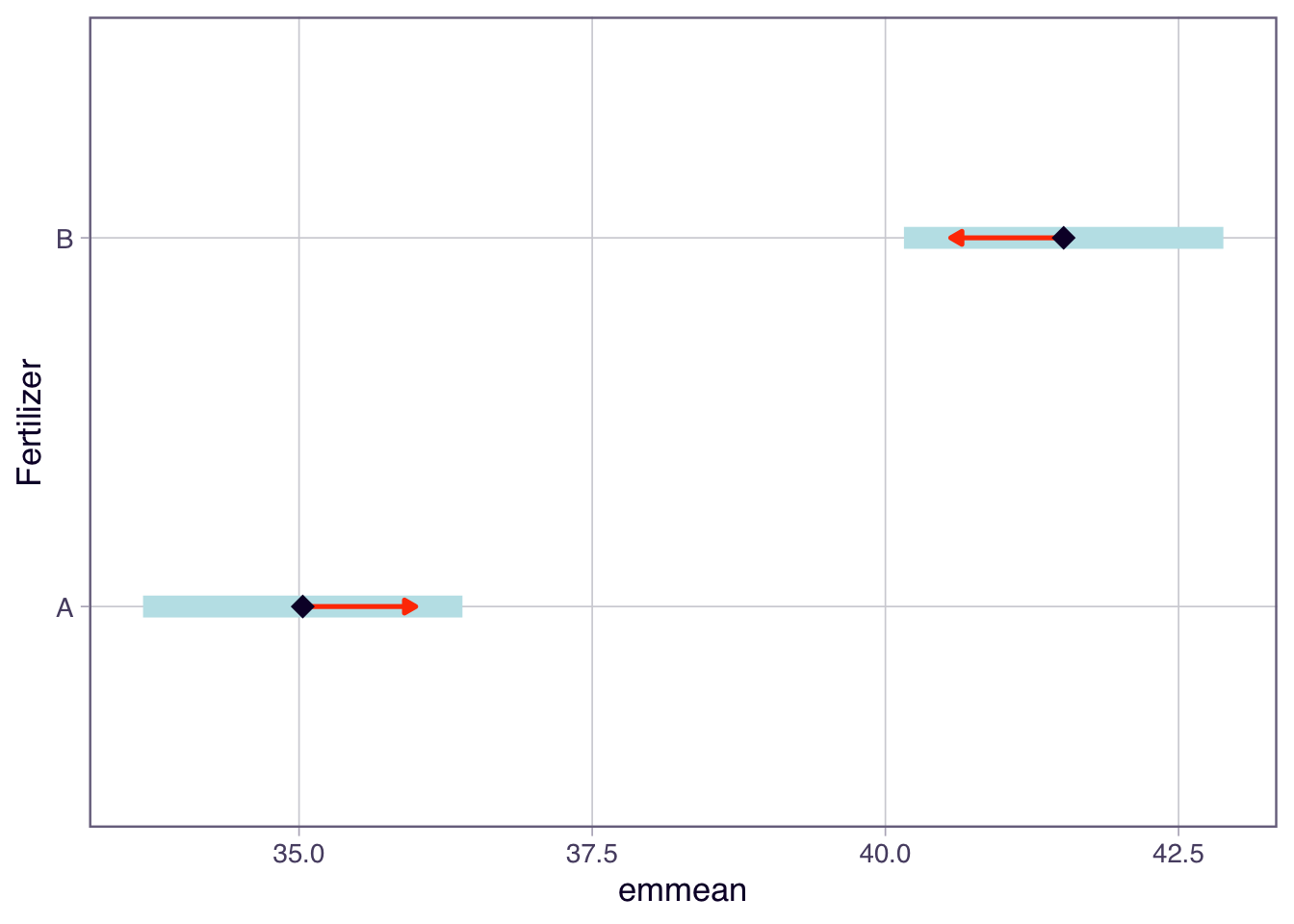
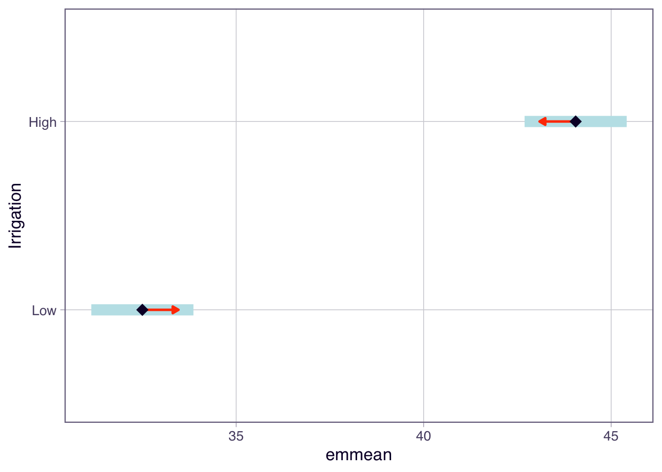
### Part B --- Visualising the effects
Now let us visualise the effects in this blocked factorial design using the `emmeans` package and its plotting functions.
```{r}
library(emmeans)
# Calculate estimated marginal means
emm <- emmeans(anova_blocked_model, ~ Fertilizer * Irrigation)

# Main effect plots using emmeans
plot(emmeans(anova_blocked_model, ~ Fertilizer),
     main = "Main Effect of Fertilizer on Crop Yield", comparisons = TRUE)
plot(emmeans(anova_blocked_model, ~ Irrigation),
     main = "Main Effect of Irrigation on Crop Yield", comparisons = TRUE)
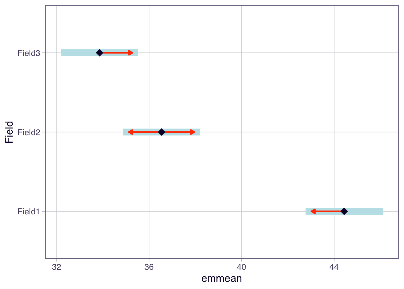
# Blocking effect plot using emmeans
plot(emmeans(anova_blocked_model, ~ Field),
     main = "Blocking Effect of Field on Crop Yield", comparisons = TRUE)
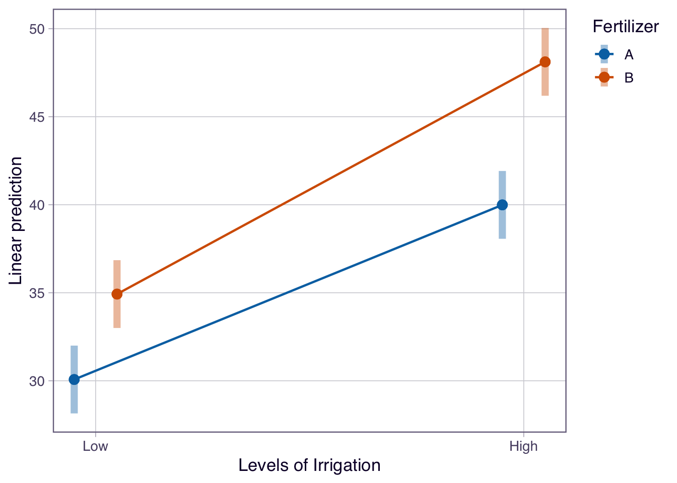
# Interaction plot using emmeans
emmip(anova_blocked_model, Fertilizer ~ Irrigation,
      main = "Interaction between Fertilizer and Irrigation on Crop Yield", CIs = TRUE)
```
> Describe the main effects and interaction effects observed in the plots above. How do these visualisations help in understanding the effects of Fertilizer and Irrigation on crop yield?
Note: We usually do not plot blocking effects as they are not of primary interest, but it can be useful to check for large differences between blocks.
Depending on our hypotheses, we may be interested in post-hoc tests for the main effects or interaction effects. If there is a significant interaction, we should focus on that rather than the main effects. We may not need to use all the plots. Always let your hypotheses guide what plots to produce.
### Part C --- Variance explained by each effect
```{r}
# Calculate variance explained by each effect
anova_summary <- summary(anova_blocked_model)
ss_total <- sum(anova_summary[[1]][, "Sum Sq"])
ss_effects <- anova_summary[[1]][, "Sum Sq"]

variance_explained <- (ss_effects / ss_total) * 100

anova_summary # ANOVA table
variance_explained # variation explained by each effect in order of the ANOVA table from top to bottom
```
> Which effect explains the most variance in crop yield? How does this information help in understanding the factors influencing crop yield?
::: {.callout-note}
## Checkpoint
You should now be able to fit a factorial ANOVA with blocking, visualise the effects using `emmeans`, and calculate the percentage of variation explained by each effect from the ANOVA table.
:::
## Wrap-up {.unnumbered}
In this tutorial, we explored factorial designs and their analysis using ANOVA. We learned about main effects, interactions, and blocking effects, and how to interpret ANOVA results in the context of factorial experiments. We also visualised these effects using ggplot2 and emmeans, enhancing our understanding of the relationships between factors and response variables in experimental designs.
### Example exam questions
1. In a 2-way factorial design with factors A (2 levels) and B (3 levels), describe how you would identify and interpret main effects and interactions using ANOVA. Provide an example of how to visualise these effects.
2. Explain the difference between a treatment design and an experimental design. Provide examples of each and discuss how they can be combined in a factorial design with blocking.
3. If you conducted a factorial experiment with blocking and found a significant interaction between two factors, how would you interpret this result? Would you still consider the main effects of each factor? Justify your answer with reference to ANOVA principles.