1 Dissimilarity Matrices and Hierarchical Clustering

In this tutorial we will use bird assemblage data from Mac Nally’s forest and woodland bird study.

Mac Nally (1989) examined forest and woodland birds along a broad environmental gradient in south-eastern Australia. The paper focused on habitat breadth, habitat position and abundance, but the same dataset is also useful for exploring whether sites with similar bird assemblages cluster together.

Here, each row is a site, and each bird species column contains an abundance or density estimate for that species at that site.

We will use hierarchical clustering to ask:

Which sites have similar bird communities?

1.1 Load packages

We need the vegan package because it contains the vegdist() function for ecological dissimilarity matrices.

library(vegan)

1.2 Load the data

The file macnally.csv contains the bird assemblage data.

If your file is in the same folder as this Quarto document use this :

macnally <- read.csv("data/macnally.csv", row.names = 1)

1.3 Examine the structure of the data

str(macnally)

'data.frame':   37 obs. of  103 variables:
 $ HABITAT : chr  "Mixed" "Gippsland Ma" "Gippsland Ma" "Gippsland Ma" ...
 $ V1GST   : num  3.4 3.4 8.4 3 5.6 8.1 8.3 4.6 3.2 4.6 ...
 $ V2EYR   : num  0 9.2 3.8 5 5.6 4.1 7.1 5.3 5.2 1.2 ...
 $ V3GF    : num  0 0 0.7 0 12.9 10.9 6.9 11.1 8.3 4.6 ...
 $ V4BTH   : num  0 0 2.8 5 12.2 24.5 29.1 28.2 18.2 6.5 ...
 $ V5GWH   : num  0 0 0 2 9.5 5.6 4.2 3.9 3.8 2.3 ...
 $ V6WTTR  : num  0 0 0 0 2.1 6.7 2 6.5 4.2 5.2 ...
 $ V7WEHE  : num  0 0 10.7 3 7.9 9.4 7.1 2.6 2.8 0.6 ...
 $ V8WNHE  : num  11.9 11.5 12.3 10 28.6 6.7 27.4 10.9 9 3.6 ...
 $ V9SFW   : num  0.4 8.3 4.9 6.9 9.2 0 13.1 3.1 3.8 3.8 ...
 $ V10WBSW : num  0 12.6 10.7 12 5 8.9 2.8 8.6 5.6 3 ...
 $ V11CR   : num  1.1 0 0 0 19.1 12.1 0 9.3 14.1 7.5 ...
 $ V12LK   : num  3.8 0.5 1.9 2 3.6 6.7 2.8 3.8 3.2 2.4 ...
 $ V13RWB  : num  9.7 11.6 16.6 11 5.7 2.7 2.4 0.6 0 0.6 ...
 $ V14AUR  : num  0 0 2.3 1.5 8.8 0 2.8 1.3 0 0 ...
 $ V15STTH : num  0 0 2.8 0 7 16.8 13.9 10.2 12.2 11.3 ...
 $ V16LR   : num  4.8 3.7 5.5 11 1.6 3.4 0 0 0.6 5.8 ...
 $ V17WPHE : num  27.3 27.6 27.5 20 0 0 16.7 0 0 0 ...
 $ V18YTH  : num  0 0 0 0 0 0 0 0 0 9.6 ...
 $ V19ER   : num  5.1 2.7 5.3 2.1 1.4 2.2 0 1.2 1.3 2.3 ...
 $ V20PCU  : num  0 0 0 0 0 0 0 0 2.8 2.9 ...
 $ V21ESP  : num  0 3.7 0 2 3.5 3.4 5.5 5.1 7.1 0.6 ...
 $ V22SCR  : num  0 0 0 0 0.7 0 0 0 0 3 ...
 $ V23RBFT : num  0 1.1 0 5 0 0.7 0 0.7 1.9 0 ...
 $ V24BFCS : num  0.6 1.1 1.5 1.4 2.7 2 3.6 0 0.6 1.2 ...
 $ V25WAG  : num  1.9 3.4 2.1 3.4 0 0 0 0 0 0 ...
 $ V26WWCH : num  0 0 0 0 0 0 0 0 0 9.8 ...
 $ V27NHHE : num  0 6.9 3 32 6.4 2.2 5.6 0 0 0 ...
 $ V28VS   : num  0 0 0 0 0 5.4 5.6 1.9 4.2 5.1 ...
 $ V29CST  : num  1.7 0.9 1.5 1.4 0 0 4.6 0 0 0 ...
 $ V30BTR  : num  12.5 0 0 0 0 0 0 0 0 0 ...
 $ V31AMAG : num  8.6 0 0 0 0 0 0 0 0 0 ...
 $ V32SCC  : num  12.5 0 0 0 0 0 0 0 0 0 ...
 $ V33RWH  : num  0.6 2.3 1.4 0 7 6.8 7.3 9.1 4.5 6.3 ...
 $ V34WSW  : num  0 5.7 24.3 10 0 0 3.6 0 0 0 ...
 $ V35STP  : num  4.8 0 3.1 4 0 0 2.4 0 0 3.5 ...
 $ V36YFHE : num  0 1.1 11.7 0 6.1 0 0 0 0 2.3 ...
 $ V37WHIP : num  0 0 0 0 0 0 0 2 3.2 0 ...
 $ V38GAL  : num  4.8 0 0 2.8 0 0 0 0 0 0 ...
 $ V39FHE  : num  26.2 0 0 0 0 0 0 0 0 0 ...
 $ V40BRTH : num  0 0 0 0 0 0 0 0 0 6 ...
 $ V41SPP  : num  0 1.1 4.6 0.8 5.4 3.4 0 2 2.6 4.2 ...
 $ V42SIL  : num  0 0 0 0 0 2.7 1.2 0 4.9 1.2 ...
 $ V43GCU  : num  0 0 0 0 0 1.4 0 2.6 1.3 0 ...
 $ V44MUSK : num  13.1 0 0 0 0 0 0 0 0 0 ...
 $ V45MGLK : num  1.7 0 0 1.4 0 0 0 0 0 0 ...
 $ V46BHHE : num  1.1 0 0 0 0 0 0 0 0 0 ...
 $ V47RFC  : num  0 0 0 0 0 0 0 0 0 0 ...
 $ V48YTBC : num  0 0 0 0 0 0 0 1.9 2.6 0 ...
 $ V49LYRE : num  0 0 0 0 0 0 0 0 0.6 0 ...
 $ V50CHE  : num  0 0 0 0 0 0 0 0 0.6 0 ...
 $ V51OWH  : num  0 0 0 0 0 0 0 0 0 0 ...
 $ V52TRM  : num  15 0 0 0 0 0 0 0 0 0 ...
 $ V53MB   : num  0 0 0 1 0 0 3.6 0 0 1.2 ...
 $ V54STHR : num  0 0 0 0 0 0 0 0 0 0 ...
 $ V55LHE  : num  0 0 0 0 0 0 0 0 0 0 ...
 $ V56FTC  : num  0 2.3 0 0 2.1 0 0 2.6 2.6 1.7 ...
 $ V57PINK : num  0 0 0 0 0 0 0 0 0 0 ...
 $ V58OBO  : num  0 0 0 0 1.4 0 0 0 0 1.2 ...
 $ V59YR   : num  0 0 0 0 0 0 0 0 0 0 ...
 $ V60LFB  : num  2.9 0 0 0 0 0 0 0 0 0 ...
 $ V61SPW  : num  0 0 0 0 0 0 0 0 0 0 ...
 $ V62RBTR : num  0 0 0 0 0 0 0 0 0 0.6 ...
 $ V63DWS  : num  0.4 0 3.5 5.5 0 0 1.8 0 0 0 ...
 $ V64BELL : num  0 0 0 0 22.1 0 0 0 0 0 ...
 $ V65LWB  : num  0 0 0 4 0 0 0 0 0 0 ...
 $ V66CBW  : num  0 0 0 0 0 0 0 0 0 0.6 ...
 $ V67GGC  : num  0 0 0 0 0 0 0 0 1.3 0 ...
 $ V68PIL  : num  0 0 0 0 0 0 0 0 1.3 0 ...
 $ V69SKF  : num  1.9 0 0 0 0 0 0 0 0 2.3 ...
 $ V70RSL  : num  6.7 0 0 0.8 0 0 0 0 0 0 ...
 $ V71PDOV : num  0 0 0 0 0 0 0 0 0 0 ...
 $ V72CRP  : num  0 0 0 0 0 0 0 0 0 0 ...
 $ V73JW   : num  0 0 0 0 0 0 0 0 0 0 ...
 $ V74BCHE : num  0 0 0 0 0 0 0 0 0 0 ...
 $ V75RCR  : num  0 0 0 0 0 0 0 0 0 0 ...
 $ V76GBB  : num  0 0 0 0 0.7 0 0 0 0.6 0 ...
 $ V77RRP  : num  4.8 0 0 0 0 0 0 0 0 0 ...
 $ V78LLOR : num  0 0 0 0 0 0 0 0 0 0 ...
 $ V79YTHE : num  0 0 0 0 0 0 0 0 0 0 ...
 $ V80RF   : num  0 0 0 0 0 1.4 0 1.9 3.2 0 ...
 $ V81SHBC : num  0 0 1.4 0 0.7 0 0 2 1.3 0.6 ...
 $ V82AZKF : num  0 0 0 0 0 0 0 0.7 0 0 ...
 $ V83SFC  : num  0 0 0 0 0 3.4 0 1.2 1.9 1.2 ...
 $ V84YRTH : num  0 0 0 0 0 0 0 0 0 0 ...
 $ V85ROSE : num  0 0 0 0 0 0 0 0.6 0 0 ...
 $ V86BCOO : num  0 0 0 0 0 0 0 0 0.6 0 ...
 $ V87LFC  : num  0 0 1.8 0 0 0 2.4 0 0 0 ...
 $ V88WG   : num  0 0 0 0 0 0 0 0 0 0 ...
 $ V89PCOO : num  1.9 0 0 0 0 0 0 0 0 0 ...
 $ V90WTG  : num  0 0 0 0 0 0 0 0 0 0 ...
 $ V91NMIN : num  0.2 0 5.8 3.1 0 0 0 0 0 0 ...
 $ V92NFB  : num  0 0 0 0 0 0 0 0 0 0 ...
 $ V93DB   : num  0 0 0 0 0 0 0 0 0 0 ...
 $ V94RBEE : num  0 0 0 0 0 0 0 0 0 0 ...
 $ V95HBC  : num  0 0 0 0 0 0 0 0 0 0 ...
 $ V96DF   : num  0 0 0 0 0 0 0 0 0 0 ...
 $ V97PCL  : num  9.1 0 0 0 0 0 0 0 0 0 ...
 $ V98FLAME: num  0 0 0 0 0 0 0 0 0 0 ...
  [list output truncated]

The first columns describe the site or habitat type. The remaining columns are bird species abundances.

ncol(macnally)

[1] 103

nrow(macnally)

[1] 37

1.4 Separate site information from species data

The HABITAT column describes the broad habitat category. The bird species data begin after the habitat column.

site_info <- macnally[, 1, drop = FALSE]
species_data <- macnally[, 2:ncol(macnally)]

head(site_info)

                 HABITAT
Reedy Lake         Mixed
Pearcedale  Gippsland Ma
Warneet     Gippsland Ma
Cranbourne  Gippsland Ma
Lysterfield        Mixed
Red Hill           Mixed

head(species_data[, 1:6])

            V1GST V2EYR V3GF V4BTH V5GWH V6WTTR
Reedy Lake    3.4   0.0  0.0   0.0   0.0    0.0
Pearcedale    3.4   9.2  0.0   0.0   0.0    0.0
Warneet       8.4   3.8  0.7   2.8   0.0    0.0
Cranbourne    3.0   5.0  0.0   5.0   2.0    0.0
Lysterfield   5.6   5.6 12.9  12.2   9.5    2.1
Red Hill      8.1   4.1 10.9  24.5   5.6    6.7

Check that the species data are numeric:

species_data <- as.data.frame(lapply(species_data, as.numeric))
rownames(species_data) <- rownames(macnally)

2 Bray-Curtis Dissimilarity

2.1 Calculate Bray-Curtis dissimilarity

Bray-Curtis dissimilarity is commonly used for ecological community data because it compares sites using species abundances.

Values range from:

0 = sites have identical assemblages
1 = sites share no species in common

Braydistance <- vegdist(species_data, method = "bray")
Braydistance

             Reedy Lake Pearcedale   Warneet Cranbourne Lysterfield  Red Hill
Pearcedale    0.6064757                                                      
Warneet       0.6192469  0.3608724                                           
Cranbourne    0.6493576  0.3458135 0.3881690                                 
Lysterfield   0.8504073  0.6274208 0.6067270  0.6679905                      
Red Hill      0.8646783  0.6974849 0.6395924  0.7012250   0.4194429          
Devilbend     0.7803703  0.5554849 0.5432526  0.5666394   0.4136546 0.4006753
Olinda        0.8728324  0.6716754 0.6963958  0.6993095   0.4338760 0.2425920
Fern Tree Gu  0.8842927  0.6968785 0.7297463  0.7147345   0.4499714 0.2855280
Sherwin       0.8476881  0.7610514 0.7041306  0.7377265   0.5725373 0.4657534
Heathcote Ju  0.8974209  0.7467483 0.6844389  0.7278521   0.5267883 0.3536222
Warburton     0.8153215  0.6633222 0.6380952  0.6420233   0.4095324 0.4015512
Millgrove     0.8219493  0.6747027 0.6293312  0.6742779   0.4030380 0.2875000
Ben Cairn     0.9311377  0.7501558 0.7619048  0.7675415   0.4907385 0.3561757
Panton Gap    0.9123711  0.7683323 0.7341635  0.7415419   0.5327723 0.3789745
OShannassy    0.9066493  0.7286796 0.6514113  0.7006459   0.5036120 0.3789901
Ghin Ghin     0.7792014  0.7436293 0.6975762  0.7337265   0.6096528 0.6017699
Minto         0.7689873  0.7439673 0.6728462  0.7266347   0.4920580 0.5161351
Hawke         0.8759055  0.6424064 0.6380060  0.6511548   0.4881841 0.3862168
St Andrews    0.8248432  0.7740822 0.7041327  0.7450822   0.4629906 0.3982202
Nepean        0.8774592  0.6449275 0.6055753  0.6705238   0.4548486 0.2912591
Cape Schanck  0.8097156  0.5754331 0.6039081  0.4468775   0.5386148 0.5345982
Balnarring    0.8849534  0.6780521 0.6940319  0.6294168   0.5442571 0.4557338
Bittern       0.7009615  0.4164188 0.3341721  0.4724653   0.5248750 0.6027579
Bailieston    0.8789157  0.8065028 0.7153797  0.7820092   0.5769116 0.5175708
Donna Buang   0.9324841  0.8249360 0.7481381  0.7836706   0.5963533 0.4998182
Upper Yarra   0.8625863  0.7412229 0.6847792  0.6992481   0.4605809 0.3933424
Gembrook      0.8512503  0.6490595 0.6087247  0.6867196   0.4669492 0.4233100
Arcadia       0.5150546  0.6724196 0.6770395  0.6935901   0.8977333 0.8852556
Undera        0.6664769  0.7503682 0.7536058  0.7271605   0.8289733 0.7920000
Coomboona     0.5987567  0.7854798 0.7184611  0.7378254   0.8642458 0.8349206
Toolamba      0.5382810  0.7081578 0.6773193  0.6555024   0.8985507 0.9092715
Rushworth     0.7271251  0.7596685 0.6550741  0.7736842   0.7194110 0.7228442
Sayers        0.7972973  0.7429010 0.6656308  0.7265176   0.5889695 0.6132670
Waranga       0.4585441  0.5790878 0.4946113  0.5544114   0.7367044 0.8186628
Costerfield   0.7079971  0.7520510 0.6940815  0.7289646   0.5651332 0.5508108
Tallarook     0.8204724  0.7350598 0.6655629  0.7013575   0.5102571 0.4989769
             Devilbend    Olinda Fern Tree Gu   Sherwin Heathcote Ju Warburton
Pearcedale                                                                    
Warneet                                                                       
Cranbourne                                                                    
Lysterfield                                                                   
Red Hill                                                                      
Devilbend                                                                     
Olinda       0.4134984                                                        
Fern Tree Gu 0.4766962 0.2191262                                              
Sherwin      0.6033313 0.4860457    0.4477504                                 
Heathcote Ju 0.5007474 0.2948987    0.3417279 0.3338252                       
Warburton    0.4322760 0.3420229    0.3545526 0.5663501    0.4297782          
Millgrove    0.4336283 0.2527538    0.2628129 0.4519950    0.3440048 0.3087515
Ben Cairn    0.5595027 0.3204164    0.2845152 0.5827034    0.3953079 0.3535584
Panton Gap   0.5174403 0.3213213    0.3285242 0.5570934    0.3577087 0.2946429
OShannassy   0.5095541 0.3168950    0.3369896 0.5488194    0.3524869 0.3564474
Ghin Ghin    0.6204506 0.6060973    0.5825666 0.5971873    0.5926561 0.6212690
Minto        0.4673546 0.5371740    0.5696203 0.6895929    0.5626719 0.4924142
Hawke        0.5231660 0.3600000    0.3729977 0.3831851    0.2821110 0.4626866
St Andrews   0.4732006 0.3973799    0.4644522 0.3684531    0.3327428 0.4698464
Nepean       0.4185047 0.3304521    0.3450915 0.4406720    0.3432432 0.4372140
Cape Schanck 0.6057348 0.5173824    0.5233918 0.6619804    0.5887407 0.5603587
Balnarring   0.4761388 0.4845554    0.4672080 0.5907007    0.5400697 0.4703462
Bittern      0.4634742 0.6365651    0.6201830 0.7380746    0.6490736 0.5515873
Bailieston   0.5800799 0.5530686    0.5880014 0.3974800    0.4930198 0.6287879
Donna Buang  0.6687276 0.4911197    0.4155392 0.6121361    0.5444532 0.4761092
Upper Yarra  0.5284752 0.3381243    0.3424460 0.4422492    0.2936015 0.4375843
Gembrook     0.4960971 0.4274643    0.4357731 0.5726496    0.4883607 0.4144411
Arcadia      0.7742811 0.9157040    0.8675000 0.7673657    0.8104596 0.8658271
Undera       0.7156948 0.8029690    0.8007430 0.5982936    0.7263374 0.7974293
Coomboona    0.7540323 0.8527936    0.8439384 0.6920366    0.7973478 0.8528736
Toolamba     0.7833633 0.9223505    0.9215686 0.8183161    0.8641053 0.9059445
Rushworth    0.7772264 0.7372774    0.7102833 0.5115269    0.6220930 0.6673219
Sayers       0.6973329 0.6306938    0.6050509 0.4228635    0.5210264 0.5603175
Waranga      0.7004464 0.8108581    0.8127191 0.7171087    0.7599392 0.6790575
Costerfield  0.6066634 0.5512857    0.5486425 0.3984652    0.4924091 0.5216125
Tallarook    0.5442159 0.4349693    0.4805035 0.4377613    0.4769614 0.4476828
             Millgrove Ben Cairn Panton Gap OShannassy Ghin Ghin     Minto
Pearcedale                                                                
Warneet                                                                   
Cranbourne                                                                
Lysterfield                                                               
Red Hill                                                                  
Devilbend                                                                 
Olinda                                                                    
Fern Tree Gu                                                              
Sherwin                                                                   
Heathcote Ju                                                              
Warburton                                                                 
Millgrove                                                                 
Ben Cairn    0.3816227                                                    
Panton Gap   0.3855517 0.2769469                                          
OShannassy   0.3444028 0.3368119  0.2825911                               
Ghin Ghin    0.5582715 0.6406751  0.6173951  0.5847382                    
Minto        0.5038482 0.5402744  0.5465995  0.5135135 0.4359377          
Hawke        0.4007807 0.4667507  0.4292282  0.4006667 0.6044699 0.6138471
St Andrews   0.3769310 0.5013809  0.4355383  0.4902887 0.6200086 0.5528872
Nepean       0.3439398 0.3925759  0.3827305  0.3727461 0.5915859 0.5844156
Cape Schanck 0.4974174 0.5930496  0.5732501  0.5413375 0.6801550 0.6878429
Balnarring   0.4707170 0.5241140  0.5177931  0.5536313 0.5880759 0.6337199
Bittern      0.5501355 0.6488696  0.6377171  0.6105395 0.5832816 0.5474478
Bailieston   0.5563840 0.6859554  0.6163009  0.6216216 0.7049837 0.7226891
Donna Buang  0.5044423 0.4251115  0.4385382  0.4623946 0.6957776 0.7023661
Upper Yarra  0.3056931 0.4362053  0.3818295  0.3122229 0.5676485 0.5537817
Gembrook     0.3818261 0.4676074  0.4231699  0.4742451 0.6147235 0.5164386
Arcadia      0.8406353 0.8512397  0.8752415  0.8753494 0.6615454 0.7160744
Undera       0.7779080 0.8388383  0.8280142  0.8191075 0.6006687 0.7253467
Coomboona    0.8022106 0.8857789  0.8703432  0.8561237 0.5982906 0.6940771
Toolamba     0.8736397 0.9242736  0.9097286  0.9084725 0.6477217 0.7306861
Rushworth    0.6482048 0.8109426  0.7065095  0.7021881 0.7348294 0.7706627
Sayers       0.5700878 0.6919459  0.6096518  0.6141220 0.6590630 0.7217631
Waranga      0.7237967 0.8701870  0.7808467  0.7616651 0.7061303 0.6873896
Costerfield  0.5090271 0.6535356  0.6079818  0.5891671 0.6383872 0.6715797
Tallarook    0.3885144 0.5861345  0.5385870  0.5510316 0.6368503 0.6410350
                 Hawke St Andrews    Nepean Cape Schanck Balnarring   Bittern
Pearcedale                                                                   
Warneet                                                                      
Cranbourne                                                                   
Lysterfield                                                                  
Red Hill                                                                     
Devilbend                                                                    
Olinda                                                                       
Fern Tree Gu                                                                 
Sherwin                                                                      
Heathcote Ju                                                                 
Warburton                                                                    
Millgrove                                                                    
Ben Cairn                                                                    
Panton Gap                                                                   
OShannassy                                                                   
Ghin Ghin                                                                    
Minto                                                                        
Hawke                                                                        
St Andrews   0.4019048                                                       
Nepean       0.3250092  0.4384376                                            
Cape Schanck 0.5188018  0.6144883 0.4728770                                  
Balnarring   0.5020548  0.6064343 0.4126552    0.4636902                     
Bittern      0.6282707  0.6575574 0.5830636    0.5561484  0.5528809          
Bailieston   0.5122736  0.4427921 0.4783821    0.7228145  0.6600326 0.6812680
Donna Buang  0.5062907  0.6192616 0.5238095    0.6848211  0.6693241 0.6990881
Upper Yarra  0.3290633  0.4195889 0.4015967    0.5533981  0.5282651 0.5963250
Gembrook     0.5176899  0.4873227 0.3702389    0.4872900  0.4995479 0.4972044
Arcadia      0.8581220  0.8015021 0.8727658    0.9031216  0.8250429 0.6776838
Undera       0.7334826  0.7128117 0.7387329    0.8740293  0.8073029 0.7920306
Coomboona    0.8269231  0.7660785 0.8082281    0.8852085  0.8404385 0.8124153
Toolamba     0.8811189  0.8617021 0.8823132    0.9039146  0.8909321 0.7617308
Rushworth    0.6383351  0.5819024 0.6711906    0.6844408  0.7441117 0.6524454
Sayers       0.4573764  0.4613791 0.5392954    0.6804277  0.6760876 0.6696680
Waranga      0.7580819  0.7262273 0.7748474    0.6913525  0.7921715 0.5439642
Costerfield  0.5119852  0.4434055 0.4995876    0.6648569  0.6510172 0.6551073
Tallarook    0.4063866  0.3479524 0.4740917    0.6066790  0.5504923 0.6338384
             Bailieston Donna Buang Upper Yarra  Gembrook   Arcadia    Undera
Pearcedale                                                                   
Warneet                                                                      
Cranbourne                                                                   
Lysterfield                                                                  
Red Hill                                                                     
Devilbend                                                                    
Olinda                                                                       
Fern Tree Gu                                                                 
Sherwin                                                                      
Heathcote Ju                                                                 
Warburton                                                                    
Millgrove                                                                    
Ben Cairn                                                                    
Panton Gap                                                                   
OShannassy                                                                   
Ghin Ghin                                                                    
Minto                                                                        
Hawke                                                                        
St Andrews                                                                   
Nepean                                                                       
Cape Schanck                                                                 
Balnarring                                                                   
Bittern                                                                      
Bailieston                                                                   
Donna Buang   0.6938776                                                      
Upper Yarra   0.5406735   0.4819326                                          
Gembrook      0.5788418   0.6313993   0.4852574                              
Arcadia       0.8367613   0.8640305   0.8322497 0.8923564                    
Undera        0.6692635   0.8449319   0.7603102 0.8135310 0.4860301          
Coomboona     0.7507898   0.8546272   0.7945493 0.8650190 0.3845216 0.3125205
Toolamba      0.8661273   0.9251674   0.8726208 0.9156449 0.3077411 0.4637830
Rushworth     0.4846871   0.8059490   0.6778257 0.6053174 0.8359034 0.7135710
Sayers        0.4089904   0.6835043   0.5870920 0.5781979 0.8322212 0.6650619
Waranga       0.7054706   0.8874082   0.7565891 0.6848160 0.6130536 0.6573686
Costerfield   0.3962930   0.6626281   0.5293083 0.5338377 0.7870564 0.6370721
Tallarook     0.5121795   0.6394558   0.4471752 0.4963161 0.8609626 0.7549789
             Coomboona  Toolamba Rushworth    Sayers   Waranga Costerfield
Pearcedale                                                                
Warneet                                                                   
Cranbourne                                                                
Lysterfield                                                               
Red Hill                                                                  
Devilbend                                                                 
Olinda                                                                    
Fern Tree Gu                                                              
Sherwin                                                                   
Heathcote Ju                                                              
Warburton                                                                 
Millgrove                                                                 
Ben Cairn                                                                 
Panton Gap                                                                
OShannassy                                                                
Ghin Ghin                                                                 
Minto                                                                     
Hawke                                                                     
St Andrews                                                                
Nepean                                                                    
Cape Schanck                                                              
Balnarring                                                                
Bittern                                                                   
Bailieston                                                                
Donna Buang                                                               
Upper Yarra                                                               
Gembrook                                                                  
Arcadia                                                                   
Undera                                                                    
Coomboona                                                                 
Toolamba     0.2675289                                                    
Rushworth    0.7728824 0.8609764                                          
Sayers       0.7899761 0.8572958 0.3555699                                
Waranga      0.6746811 0.6315256 0.4422122 0.6249683                      
Costerfield  0.7307905 0.8239679 0.3983567 0.3017514 0.5793342            
Tallarook    0.7831686 0.8734808 0.5792788 0.4818976 0.6899011   0.4121882

3 Hierarchical Clustering

3.1 Run hierarchical clustering

We will use UPGMA clustering, which is specified by method = "average" in hclust().

hc <- hclust(Braydistance, method = "average")
hc


Call:
hclust(d = Braydistance, method = "average")

Cluster method   : average 
Distance         : bray 
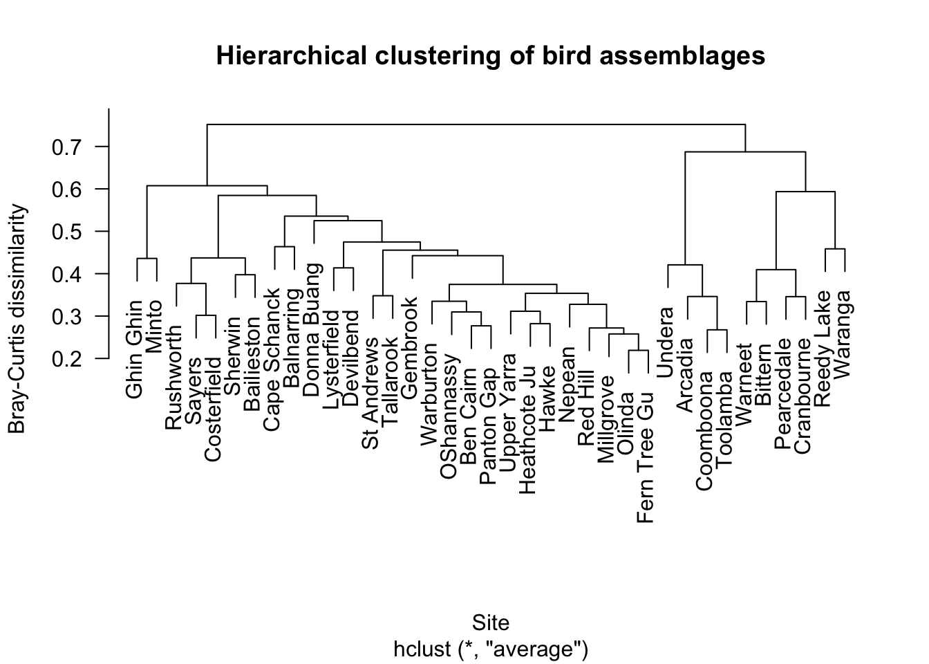
Number of objects: 37

3.2 Plot the dendrogram

plot(hc)

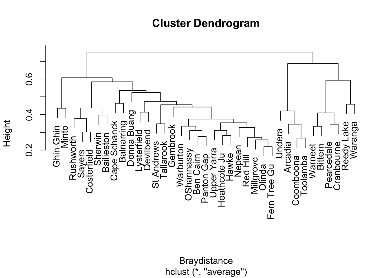
The dendrogram shows how sites are progressively joined into clusters.

Sites joined low on the dendrogram are more similar. Sites joined high on the dendrogram are more different.

3.3 Improved dendrogram with labels

plot(hc,
     las = 1,
     main = "Hierarchical clustering of bird assemblages",
     xlab = "Site",
     ylab = "Bray-Curtis dissimilarity")

3.4 Add cluster rectangles

We can draw rectangles around possible cluster solutions.

plot(hc,
     las = 1,
     main = "Cluster diagram of bird assemblages",
     xlab = "Site",
     ylab = "Bray-Curtis dissimilarity")

rect.hclust(hc, k = 2, border = "red")
rect.hclust(hc, k = 5, border = "darkgreen")

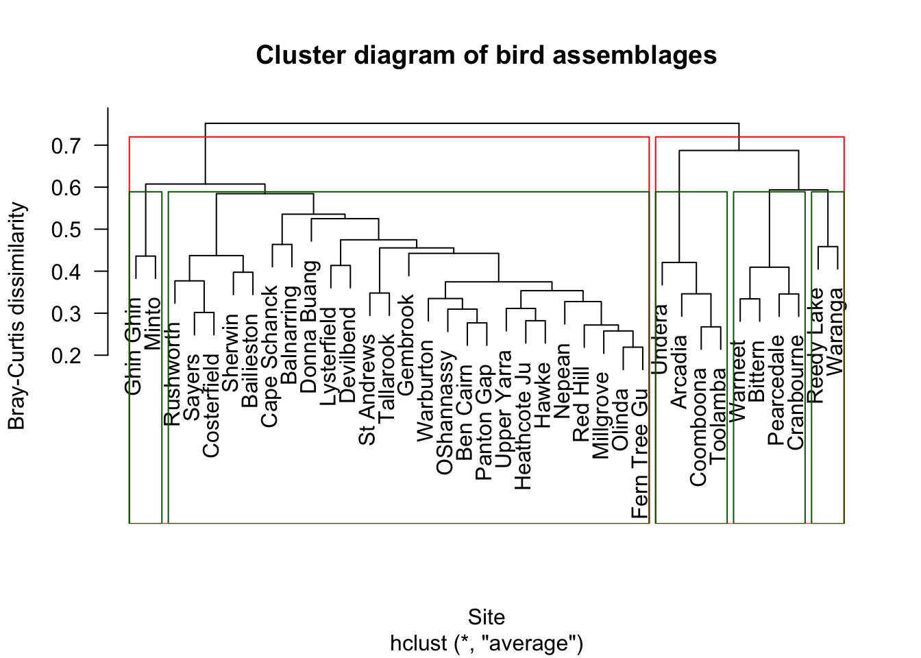
The rectangles show possible groupings:

Red rectangles = 2 broad clusters
Green rectangles = 5 finer clusters

There is no single correct number of clusters. The appropriate choice depends on the ecological question.

4 Extracting Cluster Membership

4.1 Cut the tree into clusters

Cut the tree into 5 clusters:

clusters5 <- cutree(hc, k = 5)
clusters5

  Reedy Lake   Pearcedale      Warneet   Cranbourne  Lysterfield     Red Hill 
           1            2            2            2            3            3 
   Devilbend       Olinda Fern Tree Gu      Sherwin Heathcote Ju    Warburton 
           3            3            3            3            3            3 
   Millgrove    Ben Cairn   Panton Gap   OShannassy    Ghin Ghin        Minto 
           3            3            3            3            4            4 
       Hawke   St Andrews       Nepean Cape Schanck   Balnarring      Bittern 
           3            3            3            3            3            2 
  Bailieston  Donna Buang  Upper Yarra     Gembrook      Arcadia       Undera 
           3            3            3            3            5            5 
   Coomboona     Toolamba    Rushworth       Sayers      Waranga  Costerfield 
           5            5            3            3            1            3 
   Tallarook 
           3

Add the cluster identity back to the site information:

cluster_summary <- data.frame(
  Site = rownames(macnally),
  Habitat = macnally$HABITAT,
  Cluster = clusters5
)

cluster_summary

                     Site      Habitat Cluster
Reedy Lake     Reedy Lake        Mixed       1
Pearcedale     Pearcedale Gippsland Ma       2
Warneet           Warneet Gippsland Ma       2
Cranbourne     Cranbourne Gippsland Ma       2
Lysterfield   Lysterfield        Mixed       3
Red Hill         Red Hill        Mixed       3
Devilbend       Devilbend        Mixed       3
Olinda             Olinda        Mixed       3
Fern Tree Gu Fern Tree Gu Montane Fore       3
Sherwin           Sherwin Foothills Wo       3
Heathcote Ju Heathcote Ju Montane Fore       3
Warburton       Warburton Montane Fore       3
Millgrove       Millgrove        Mixed       3
Ben Cairn       Ben Cairn        Mixed       3
Panton Gap     Panton Gap Montane Fore       3
OShannassy     OShannassy        Mixed       3
Ghin Ghin       Ghin Ghin        Mixed       4
Minto               Minto        Mixed       4
Hawke               Hawke        Mixed       3
St Andrews     St Andrews Foothills Wo       3
Nepean             Nepean Foothills Wo       3
Cape Schanck Cape Schanck        Mixed       3
Balnarring     Balnarring        Mixed       3
Bittern           Bittern Gippsland Ma       2
Bailieston     Bailieston Box-Ironbark       3
Donna Buang   Donna Buang        Mixed       3
Upper Yarra   Upper Yarra        Mixed       3
Gembrook         Gembrook        Mixed       3
Arcadia           Arcadia River Red Gu       5
Undera             Undera River Red Gu       5
Coomboona       Coomboona River Red Gu       5
Toolamba         Toolamba River Red Gu       5
Rushworth       Rushworth Box-Ironbark       3
Sayers             Sayers Box-Ironbark       3
Waranga           Waranga        Mixed       1
Costerfield   Costerfield Box-Ironbark       3
Tallarook       Tallarook Foothills Wo       3

4.2 How many sites are in each cluster?

table(cluster_summary$Cluster)


 1  2  3  4  5 
 2  4 25  2  4

4.3 Do clusters correspond to habitat types?

table(cluster_summary$Habitat, cluster_summary$Cluster)

              
                1  2  3  4  5
  Box-Ironbark  0  0  4  0  0
  Foothills Wo  0  0  4  0  0
  Gippsland Ma  0  4  0  0  0
  Mixed         2  0 13  2  0
  Montane Fore  0  0  4  0  0
  River Red Gu  0  0  0  0  4

This table helps us ask whether bird assemblage clusters correspond to habitat categories.

If sites from the same habitat type mostly fall into the same cluster, then bird communities are strongly structured by habitat.

If habitat types are spread across several clusters, then bird assemblages may be influenced by other factors as well.

5 Optional: Compare Clustering Methods

5.1 Single linkage

hc_single <- hclust(Braydistance, method = "single")

plot(hc_single,
     las = 1,
     main = "Single linkage clustering",
     xlab = "Site",
     ylab = "Bray-Curtis dissimilarity")

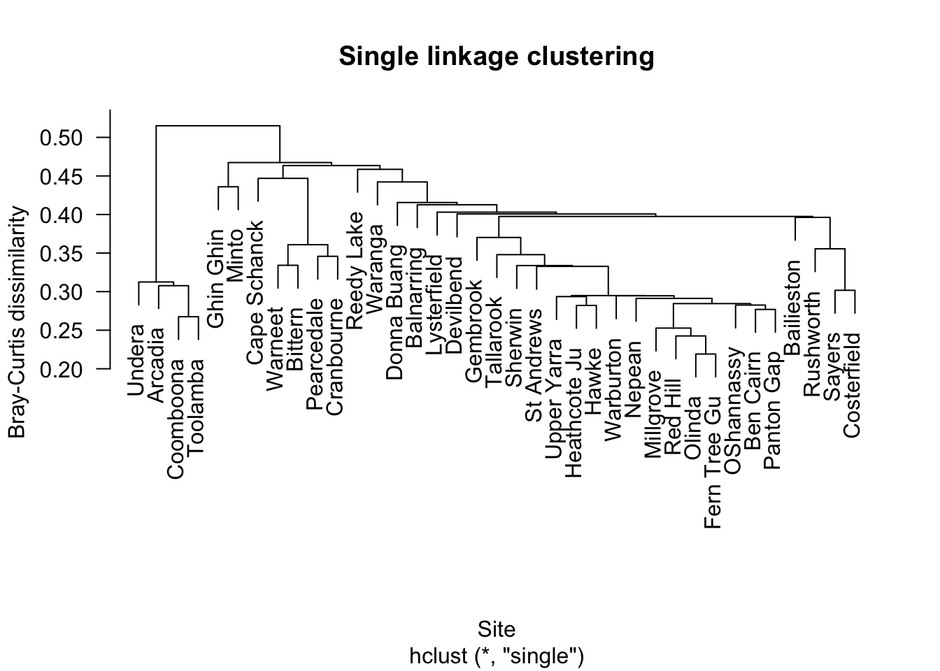
Single linkage can produce chaining, where sites are joined one at a time into long strings.

5.2 Complete linkage

hc_complete <- hclust(Braydistance, method = "complete")

plot(hc_complete,
     las = 1,
     main = "Complete linkage clustering",
     xlab = "Site",
     ylab = "Bray-Curtis dissimilarity")

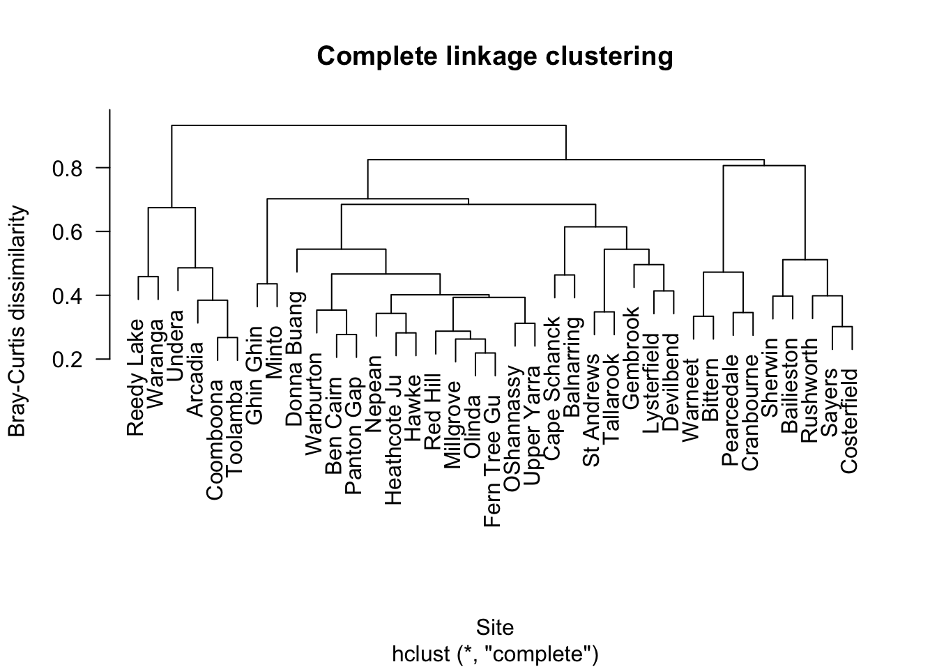
Complete linkage tends to produce more compact clusters.

5.3 Average linkage

hc_average <- hclust(Braydistance, method = "average")

plot(hc_average,
     las = 1,
     main = "Average linkage clustering / UPGMA",
     xlab = "Site",
     ylab = "Bray-Curtis dissimilarity")

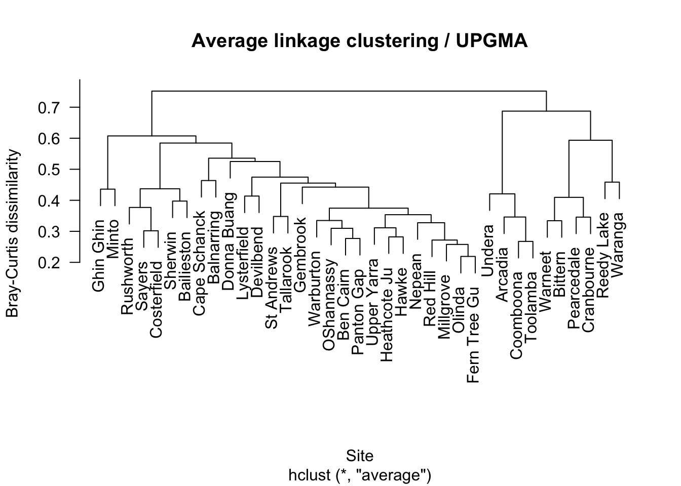
Average linkage is often a useful compromise and is commonly used in ecological community analysis.

6 Student Questions

6.1 Question 1

What does Bray-Curtis dissimilarity measure in this analysis?

Answer guide

It measures how different two sites are in their bird assemblages, based on species abundances.

A value near 0 means sites are very similar. A value near 1 means sites are very different.

6.2 Question 2

What does it mean when two sites join low on the dendrogram?

Answer guide

They have similar bird assemblages.

The lower the joining point, the smaller the dissimilarity between the sites.

6.3 Question 3

Why might we compare 2-cluster and 5-cluster solutions?

Answer guide

A 2-cluster solution shows very broad differences among sites.

A 5-cluster solution shows finer ecological structure.

The best level depends on whether we want a broad or detailed interpretation.

6.4 Question 4

Why might clusters not perfectly match habitat categories?

Answer guide

Bird assemblages may respond to more than broad habitat type.

They may also be influenced by vegetation structure, geographic location, resource availability, disturbance, or species interactions.

7 Key Take-home Message

Hierarchical clustering groups sites according to similarity in bird assemblages.

For the Mac Nally bird data, this lets us explore whether woodland and forest sites form distinct community types.

The method does not tell us the “true” number of ecological groups. Instead, it gives a visual and quantitative way to explore patterns in community composition.