Apply the steps for hypothesis testing from lectures
Learn how to interpret statistical output
Before you begin
Turn off GitHub Copilot
It is quite important that you go through this lab without using GitHub Copilot.
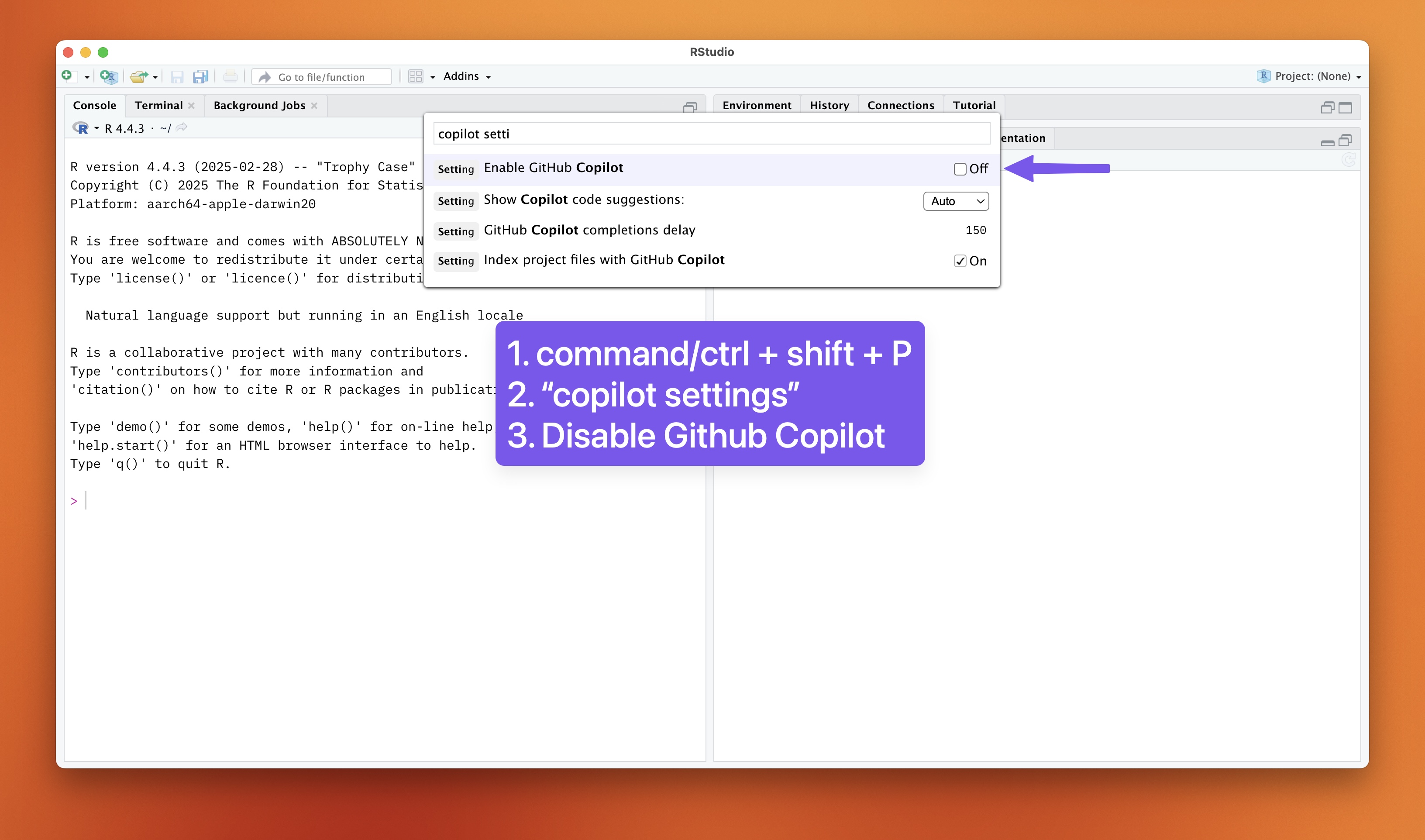
It is a great tool, but it can lead to dependency on AI assistance rather than developing your statistical reasoning skills. Turn it on again after the lab if you want to use it for other projects. GitHub Copilot is also not allowed in the mid-semester exam (where you will be required to apply statistics in R, under exam conditions). To turn off GitHub Copilot:
Open the Command Palette (Ctrl+Shift+P or Cmd+Shift+P on Mac)
Type “Copilot” and select “GitHub Copilot: Enable Copilot” to disable it (make sure the checkbox is unchecked).
You can also disable it in the Settings by going to Tools > Global Options > GitHub Copilot and unchecking the “Enable GitHub Copilot” option.
Disable GitHub Copilot. Click to enlarge.
Your Quarto document
Create your Quarto document and save it as Lab-06.Qmd or similar. The following data files are required:
Finally, try to complete today’s lab exercises in pairs and try out pair programming, where one person writes the code and the other person reviews each line as it is written. You can swap roles every 10 minutes or so. Showing someone how you code is an excellent way to learn, and you will be surprised how much you can learn from each other.
Exercise 1: barley (walk-through)
Background
An experiment was designed to compare two varieties of spring barley. Thirty four plots were used, seventeen being randomly allocated to variety A and seventeen to variety B. Unfortunately five plots were destroyed. The yields (t/ha) from the remaining plots were as they appear in the file Barley.csv.
Instructions
First, quickly explore the data; then, utilise the HATPC process and test the hypothesis that the two varieties give equal yields, assuming that the samples are independent.
HATPC:
Hypothesis
Assumptions
Test (statistic)
P-value
Conclusion
NoteLevel of significance
The level of significance is usually set at 0.05. This value is generally accepted in the scientific community and is also linked to Type 2 errors, where choosing a lower significance increases the likelihood of failing to reject the null hypothesis when it is false.
Data exploration
First we load the data and inspect its structure to see if it needs to be cleaned or transformed. The glimpse() function is a tidy version of str() that provides a quick overview of the data that focuses on the variables, ignoring data attributes.
Try to compare str() and glimpse() to see what the differences are.
barley <- readr::read_csv("data/Barley.csv") # packagename:: before a function lets you access a function without having to load the whole library firstdplyr::glimpse(barley)
The Variety column is a factor with two levels, A and B, but it is defined as a character. We can convert it to a factor using the mutate() function from the dplyr package, but it is not necessary for the t-test since R will automatically convert it to a factor.
Quickly preview the data as a plot to see if there are any trends or unusual observations.
barley %>%ggplot(aes(x = Variety, y = Yield)) +geom_boxplot()
A trained eye will anticipate that the data may not meet the assumption of equal variance; however, we will test this assumption later. Otherwise, there appear to be no unusual observations in the data.
Hypothesis
What are the null and alternative hypotheses? We can use the following notation:
\[H_0: \mu_A = \mu_B\]\[H_1: \mu_A \neq \mu_B\]
where \(\mu_A\) and \(\mu_B\) are the population means of varieties A and B, respectively.
It is important that when using mathematical symbols to denote the null and alternative hypotheses, you should always define what the symbols mean. Otherwise, the reader may not understand what you are referring to.
The equations above are written in LaTeX, a typesetting system that is commonly used in scientific writing. You can learn more about LaTeX here. The raw syntax used to write the equations are shown below:
$$H_0: \mu_A = \mu_B$$$$H_1: \mu_A \neq \mu_B$$
Why do we always define the null and alternative hypotheses? In complex research projects or when working in a team, it is important to ensure that everyone is on the same page. By defining the hypotheses, you can avoid misunderstandings and ensure that everyone is working towards the same goal as the mathematical notation is clear and unambiguous.
Assumptions
Normality
There are many ways to check for normality. Here we will use the QQ-plot. Use of ggplot2 is preferred (as a means of practice) but since we are just exploring data, base R functions are not a problem to use.
ggplot(barley, aes(sample = Yield)) +stat_qq() +stat_qq_line() +facet_wrap(~Variety) #facet_wrap ensures there are separate plots for each variety rather than one plot with all the data in Yield
par(mfrow =c(1, 2))qqnorm(barley$Yield[barley$Variety =="A"], main ="Variety A") # square brackets to subset the data by varietyqqline(barley$Yield[barley$Variety =="A"])qqnorm(barley$Yield[barley$Variety =="B"], main ="Variety B")qqline(barley$Yield[barley$Variety =="B"])
Question: Do the plots indicate the data are normally distributed?
Answer: Yes, the data appear to be normally distributed as the QQ-plot shows that the data points are close to the line.
Homogeneity of variance
From the boxplot, we can see that there is some indication that the variances are not equal. We can test this assumption using a F-test, Bartlett’s test or Levene’s test; here we will just use Bartlett’s test (look up the different tests for equal variance and pros and cons of each).
\(H_0: \text{Variance is equal across all groups}\)\(H_1: \text{Variance is NOT equal across all groups}\)
bartlett.test(Yield ~ Variety, data = barley)
Bartlett test of homogeneity of variances
data: Yield by Variety
Bartlett's K-squared = 14.616, df = 1, p-value = 0.0001318
Question: Does the Bartlett’s test indicate the two groups have equal variances? What effect will that have on the analysis?
Answer: The two groups have unequal variance (Bartlett’s test: \(X^2 = 14.6\), \(p < 0.01\)). This means that we will need to use the Welch’s t-test, which does not assume equal variances.
Test statistic
We can now calculate the test statistic using the t.test() function in R. Since the variances are unequal, we do not have to specify the var.equal argument – the default test for t.test() is the Welch’s t-test which does not assume equal variances.
t.test(Yield ~ Variety, data = barley)
Welch Two Sample t-test
data: Yield by Variety
t = -4.9994, df = 19.441, p-value = 7.458e-05
alternative hypothesis: true difference in means between group A and group B is not equal to 0
95 percent confidence interval:
-0.9293569 -0.3814274
sample estimates:
mean in group A mean in group B
4.052941 4.708333
P-value
Since the p-value is < 0.05, we can reject the null hypothesis that the mean yield of both varieties is equal.
Conclusion
The conclusion needs to be brought into the context of the study. In a scientific report or paper, you would write something like this:
The mean yield of barley variety A was significantly different from that of variety B (\(t = -5.0\), \(df = 19.4\), \(p < 0.01\)).
Exercise 2: plant growth
Background
In a test of a particular treatment aimed at inducing growth, 20 plants were grouped into ten pairs so that the two members of each pair were as similar as possible. One plant of each pair was chosen randomly and treated; the other was left as a control. The increases in height (in centimetres) of plants over a two-week period are given in the file Two week plant heights. We wish to compare whether the treatment is actually inducing improved growth, as compared to the control.
Instructions
Here, we have two samples, and the samples are paired as it is a before-after experiment (the data are NOT independent). So we’d like to conduct a paired t-test.
For paired t-tests the analysis is performed as a 1-sample t-test on the difference between each pair so the only assumption is the normality assumption.
Copy the structure below and perform your analysis in your document.
## Exercise 2: plant growth### Data exploration### Hypothesis### Assumptions#### Normality#### Homogeneity of variance (if required)### Test statistic### P-value### Conclusion
Note 1. The data is not tidy. The code below will convert the data to the long format and assign it to tidy_plant which can be useful for ggplot. Note 2. The data are paired so we look at the difference when testing hypotheses. Note 3. We cannot perform a paired t.test on data in long format - this is to ensure the data remains “tied/paired” i.e. Floris before heart rate doesn’t get mixed up with Liana’s after heart rate.
A new filtering process was installed at a dam which provided drinking water for a nearby town. To check on its success, a number of water samples were taken at random times and locations in the weeks before and after the process was installed. The following are the turbidity values (units = NTU) of the water samples.
Instructions
Now we consider further examples of a two-sample t-test, but where the assumption of equal variance and normality may not be met for the raw data. Sometimes after applying a data transformation the analysis can proceed assuming equal variances – but always check after a data transformation.
For data transformation, you may need to create a new variable in your dataset to store the transformed data. For example, to create a new variable TurbLog10 that stores the log10 transformed turbidity values, you can use the following code:
To interpret the results for your conclusions, you may need to back-transform the mean and/or confidence interval values. To back transform log10 data you use:
\[10^{\text{mean or CI}}\]
To back-transform natural log, loge, you use:
\[e^{\text{mean or CI}}\]
Bonus take home exercises
Use the HATPC framework to answer the following questions
Hypothesis
Assumptions
Test (statistic)
P-value
Conclusion
Exercise 1: Tooth growth
Tooth GRowth is an inbuilt dataset that shows the effect of vitamin c in Guinea pig tooth growth. It has three variables:
len = tooth length
supp = type of supplement (Orange juice or ascorbic acid)
dose = mg/day given to the guinea pigs
head(ToothGrowth)str(ToothGrowth)
Using the HATPC framework, test whether the type of supplent affects tooth length.
Exercise 2: Adelie penguin bill length
For this exercise, we will be using a subset of the palmer penguins dataset.