Chi-squared tests
The chi-squared distribution (where chi is pronounced ‘ky’) is a very widely used distribution in statistics. Its symbol is \(\chi^2\). It has MANY applications. Here we will consider only two of these applications – tests of agreement with expected outcomes, and contingency tables.
Notes on the \(\chi^2\) Distribution
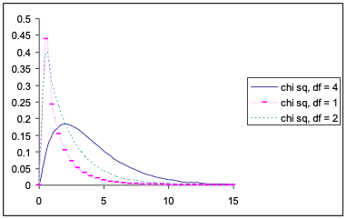
The density function for a \(\chi^2\) distribution is positively skewed, that is, it has a long tail to the right. The typical shape of the \(\chi^2\) density function is that shown for the 4 df case in Figure 7.1 below. When df is very low e.g. 1 or 2, the curve changes shape dramatically. When df are very large (say greater than 100), the \(\chi^2\) distribution approaches the shape (and properties) of a normal distribution.
The mean and variance of a \(\chi^2\) variable are simple functions of the degrees of freedom of the distribution. If we express the general degrees of freedom as \(\nu\) (Greek n), then
- Mean of \(\chi^2\) variable = \(\nu\) (i.e. mean = df)
- Variance of \(\chi^2\) variable = \(2\nu\) (i.e. variance = twice the df)
Critical values of a \(\chi^2\) distribution are given in the \(\chi^2\) probability table that appears as Appendix A.5.
Testing Agreement of Frequency Data with Expectation Models
Steps in Chi-Squared Tests of Agreement
The process for performing a goodness of fit test is the similar to that of the other hypothesis tests you have encountered thus far, that is,
Choose an appropriate hypothesis test for the type of data you have, and the type of question you’re asking.
Choose the level of significance for the test.
Write null and alternate hypotheses. Here (as for normality tests) the null hypothesis is always that the data can be assumed to follow the distribution under consideration.
Calculate the expected values. To do this, we assume that the null hypothesis is true and generate the expected values accordingly
Check the assumptions or requirements of the test. For observed versus expected chi square goodness of fit tests, the requirements of the test are that a) no cell should have an expected value of less than 1 and b) no more than 20% of cells should have expected values less than 5. To overcome either of these problems, we tend to collapse cells together before calculating the test statistic – however there are alternative tests designed to accommodate these situations.
Calculate the test statistic and degrees of freedom.
Obtain the P-value.
Draw a statistical conclusion, and use this to generate a biological conclusion.
Examples: Testing Whether Outcomes are Equally Probable
EXAMPLE 1
Sometimes the simplest form of hypothesis is that different outcomes are equally probable. For example, we expect that when a “fair” coin is tossed that the heads and tails outcomes are equally probable. However, we would see different results if the coin is biased and we can conduct a formal hypothesis test to see whether the outcomes are deviating significantly from our expectation of a “fair” coin.
EXAMPLE 2 (from Mead et al, 2003)
Suppose that 40 testers were asked to compare four different cheeses produced by different procedures and identified only by the letters A, B, C, D. Assume that each tester makes one choice and the preferences were as follows.
| Cheese | First preference |
|---|---|
| A | 5 |
| B | 7 |
| C | 18 |
| D | 10 |
| Total | 40 |
We might suspect that this shows an overall preference for C. To test the simple model that testers are equally likely to prefer A, B, C, or D, we would calculate the expected frequency for each cheese to be preferred as the total number of testers divided by 4 = 40/4 = 10. Then we calculate:
\[\chi^2_{obs}=\frac{(5-10)^2}{10}+ \frac{(7-10)^2}{10}+ \frac{(10-10)^2}{10} =9.80\]
This time we have four frequencies with one overall restriction that they total 40, and so there are 3 df. The 5% point of the \(\chi^2\) distribution on 3df is 7.82, so the unevenness of the preferences is significant (given that the \(\chi^2_{obs}\) value of 9.80 is greater than the \(\chi^2_{crit}\) value of 7.82. The evidence suggests that the model of equally likely choices is incorrect. [Equivalently, we could produce a chi-squared probability via =CHISQ.DIST.RT(9.80,3) in Excel which returns P = 0.0203. We reject H0 since \(P < 0.05\))
To assess the extent to which it is the preference for cheese C that contradicts the model, we might decide to do a further test to compare whether the preference for C only is different to the preference for all the other cheeses. In a model of likely choices, our expected values are C = 10 and all other = 30. We observed C = 18, and all other = 22. You can proceed with the test as per above starting with
\[ \chi^2_{obs}=\frac{(18-10)^2}{10}+ \frac{(22-30)^2}{30} =…\text{etc.}\]
Example: Testing Whether Outcomes are in Expected Proportions
(from Mead et al, 2003)
A total of 560 primula plants were classified by the type of leaf (flat or crimped) and the type of eye (normal or Primrose Queen).
The figures obtained for the primula plants follow.
| Normal eye | Primrose Queen eye | Total | |
|---|---|---|---|
| Flat leaves | 328 | 122 | 450 |
| Crimped leaves | 77 | 33 | 110 |
| Total | 405 | 115 | 560 |
On the hypothesis of a Mendelian 3:1 ratio, we would expect, for each characteristic, 3/4 of the total 560 observation in the first class of the characteristic and the remaining 1/4 in the second class. Further, this model predicts that 3/4 of the flat-leaved plants should have normal eyes, resulting in 3/4 \(\times\) 3/4 of all the plants or 9/16 with flat leaves and normal eyes; the remaining 3/4 of the flat-leaved plants, which is 1/4 \(\times\) 3/4or 3/16, should have Primrose Queen eyes. Similarly, 3/16 of the plants should have crimped leaves and normal eyes; and 1/16 crimped leaves and Primrose Queen eyes.
The calculation of these expected or predicted proportions is shown below.
| Normal eye | Primrose Queen eye | |
|---|---|---|
| Flat leaves | 3/4 x 3/4 = 9/16 | 1/4 x 3/4 = 3/16 |
| Crimped leaves | 3/4 x 1/4 = 3/16 | 1/4 x 1/4 = 1/16 |
Hence, the hypothesis predicts ratios of 9:3:3:1 for the four classes (flat normal: flat Primrose Queen: crimped normal: crimped Primrose Queen). The expected frequencies are calculated as 9/16, 3/16, 3/16, and 1/16 of 560, producing 315, 105, 105, and 35.
The observed and expected frequencies are summarized in the table below.
| Normal eye | Primrose Queen eye | |
|---|---|---|
| Flat leaves | 328 (315) | 122 (105) |
| Crimped leaves | 77 (105) | 33 (35) |
\[ \begin{split} \chi^2_{obs} &= \frac{(328-315)^2}{315}+ \frac{(122+105)^2}{105}+ \frac{(77-105)^2}{105}+ \frac{(33-35)^2}{35} \\ &= 0.54 + 2.75 + 7.47 + 0.11 \\ &= 10.77. \end{split} \] We compare 10.77 with the 5% point of the \(\chi^2\) distribution on 3df (7.82). We conclude that the 9:3:3:1 model is not acceptable.
See pp. 332-333 of Mead et al, 2003 for what to do next… after rejecting the model.
Contingency Tables
Example: (2 x 2) Contingency Table
Consider an experiment in which two surgical procedures are to be compared by observing the recovery rates of animals receiving either Procedure 1 or Procedure 2. Twenty animals were randomly allocated to receive Procedure 1 and twenty animals to receive Procedure 2.
| Yes | No | Total | |
|---|---|---|---|
| Procedure 1 | 2.05 | 6 | 20 |
| Procedure 2 | 1.37 | 12 | 20 |
| Total | 20 | 18 | 40 |
This is one form of a 2x2 contingency table, since there are two rows and two columns (ignoring the totals). It appears that Procedure 1 leads to a higher recovery rate. Is this due to chance?
Solution: We will perform a statistical hypothesis test:
H0: There is no difference in the true recovery rates for animals on either procedure.
H1: The recovery rates do differ.
In terms of parameters, let p1 be the probability that an animal recovers under Procedure 1, and p2 the probability that an animal recovers under Procedure 2. Then the hypotheses are equivalent to
\[ H_0: p_1 = p_2 H_1: p_1 \neq p_2 \]
Estimates of individual recovery rates are \(\hat p = 14/20 = 0.7\) and \(\hat p = 8/20 = 0.4\). Is this difference due to chance?
If H0 is true, there is a common recovery rate (which we label p). Assuming H0 is true, the best estimate of p is
\[ \hat p = \frac{14 +8}{20+20}= \frac{22}{40}=0.55 \]
So the expected frequency (under H0) of recoveries for Procedure 1 would be $20 /40 = 20 = 11 $ animals. In general this can be written as: \[ \text{Expected Frequency} = \frac{( \text{row total})\times (\text{Column total})}{\text{Grand Total}} \] So the expected frequencies for the cells in the table are: \[ \begin{split} \text{Procedure 1, Recovered:}\ \frac{20 \times 22}{40} &= 11\\ \text{Procedure 1, Not recovered:}\ \frac{20 \times 18}{40} &=9 \\ \text{Procedure 2, Recovered:}\ \frac{20 \times 22}{40} &= 11\\ \text{Procedure 2, Not recovered:}\ \frac{20 \times 18}{40} &=9 \end{split} \] Expected frequencies are written on the contingency table in parentheses, allowing comparisons with observed frequencies:
| Yes | No | Total | |
|---|---|---|---|
| Procedure 1 | 14 (11) | 6 (9) | 20 |
| Procedure 2 | 8 (11) | 12 (9) | 20 |
| Total | 20 | 18 | 40 |
The table shows observed (and expected) frequencies. The \(\chi^2\) test statistic is then calculated using: \[ \begin{split} \chi^2 &=\sum \frac{\text{(Observed - expected)}^2}{\text{Expected}}\\ &=\frac{(14-11)^2}{11}+\frac{(6-9)^2}{9}+ \frac{(8-11)^2}{11}+\frac{(12-9)^2}{9}\\ &= 3.64 \end{split} \] Large values of \(\chi^2\) indicate discrepancies between observed and expected frequencies, i.e. large values indicate that H0 should be rejected in favour of H1.
The df of this \(\chi^2\) test is 1 for a \(2 \times 2\) contingency table. In general, >df = (number of rows - 1) x (number of columns - 1)
If H0 is true, the observed \(\chi^2\) is just one observation from a \(\chi^2\) distribution with 1 df:
Since \(P =P(\chi^2_1>3.64)=0.056\), there is (just) not sufficient evidence to reject H0. Thus, while Procedure 1 has a higher recovery rate, it just fails to reach statistical significance. At this stage, the difference in individual recovery rates appears to be chance. Increasing the numbers of animals in a new experiment will determine the question with higher precision.
Example: (4 x 3) Contingency Table
The second example is a 43 contingency table. Three vaccines for a disease were compared with a control. The number of animals with no, mild, and severe infection was recorded after 24 months. Data were recorded in the following table:
| Vaccine | No | Mild | Severe | Total |
|---|---|---|---|---|
| Control | 100 (137.3) | 71 (42.6) | 29 (20.1) | 200 |
| A | 146 (133.9) | 32 (41.6) | 17 (19.6) | 195 |
| B | 149 (132.5) | 28 (41.2) | 16 (19.3) | 193 |
| C | 146 (137.3) | 37 (42.6) | 17 (20.1) | 200 |
| Total | 541 | 168 | 79 | 788 |
The table shows observed (and expected) frequencies.
We test H0 that there is no association between disease status and vaccination given, i.e. all vaccinations have equal effectiveness.
Assuming H0 is true, the expected frequencies are calculated as follows:
e.g. Expected frequency for an animal in the Control, No disease group: \[ \frac{\text{row total}\times \text{column total}}{\text{grand total}} = \frac{200 \times 541}{788} =137.3 \]
As before, the test statistic is $^2 = $ and this will have (4-1)\(\times\)(3-1) = 6 df.
Pearson chi-squared value is 45.22 with 6 df.
Probability level (under null hypothesis) p < 0.001
The other available method is known as the maximum likelihood (ML) method. The two answers are usually very similar:
Likelihood chi-squared value is 43.34 with 6 df.
Probability level (under null hypothesis) p < 0.001
The ML \(\chi^2\) is calculated as follows: \[ \chi^2=2\sum Observed \times ln(\frac{Observed}{Expected} ) \]
The degrees of freedom are (r – 1)(c – 1) as before, where r and c are the numbers of rows and columns respectively.
In general, the \(\chi^2\) approximation should only be used if the sample size is relatively large. As a general rule, there should be few expected frequencies below 5 and none below 1.0. Most packages will print out a warning when this occurs. Some situations allow exact probabilities to be calculated, but we will not pursue that in this course.
An example of low numbers would be the following, (these are basically 1/10th the numbers in the previous example):
| Vaccine | No | Mild | Severe | Total |
|---|---|---|---|---|
| Control | 10 | 7 | 3 | 20 |
| A | 15 | 3 | 2 | 20 |
| B | 15 | 3 | 2 | 20 |
| C | 15 | 4 | 2 | 21 |
| Total | 55 | 17 | 9 | 81 |